Research Studies

There are many metrics used to quantify the impact of surface ozone on human and vegetation health or assess the performance of atmospheric chemistry models. Surface ozone concentrations vary depending on the time of day, and some metrics focus on just the hour with the highest ozone concentration, while others consider ozone over an 8, 12, or 24 hour period. Consequently, changes in the daily cycle of ozone concentrations over time lead to different trends depending on which metric is considered.

We use a high resolution global atmospheric chemistry model simulation to investigate how the magnitude of the daily cycle in ozone is changing in different regions of the world in response to changes in NOx emissions. The model simulation shows good agreement with the NO2 trends seen by the OMI satellite instrument and with the changes in the daily ozone cycle observed at rural sites in the eastern United States. This gives us more confidence to apply the model to other regions where sufficient surface data is not available. Our simulation predicts that the magnitude of the daily variability in surface ozone increased from the 1980s to present in regions such as China where NOx emissions increased, while the magnitude decreased where emissions decreased. Consequently, both positive and negative trends in peak surface ozone concentrations are stronger than the trends in ozone averaged over the whole day.

Citation:
Strode, S.A., Ziemke, J.R., Oman, L.D., Lamsal, L.N., Olsen, M.A. and Liu, J., 2019. Global changes in the diurnal cycle of surface ozone. Atmospheric Environment, 199, pp.323-333, DOI: https://doi.org/10.1016/j.atmosenv.2018.11.028.

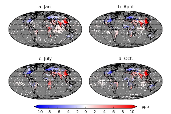
Figure 1. The change in the peak-to-peak magnitude of the diurnal cycle of surface ozone for 2006-2015 versus 1980-1989 in the MERRA-2 GMI simulation.

Effects of Greenhouse Gas Increase and Stratospheric Ozone Depletion on Stratospheric Mean Age of Air in 1960-2010

The stratospheric mean age of air is the average time that an air parcel spends when it transports from troposphere to stratosphere. The mean age has been robustly shown to decrease in climate simulations of the recent past, indicating an acceleration of the stratospheric transport circulation. The decrease in mean age is caused by two major anthropogenic forcings: greenhouse gas (GHG) increase and stratospheric ozone depletion. However, the relative importance of these two drivers remains uncertain.

This study separates the relative impacts of greenhouse gas increase and stratospheric ozone depletion on stratospheric mean age of air in 1960-2010 using the Goddard Earth Observing System Chemistry-Climate Model (GEOSCCM). We conducted a set of experiments using a coupled ocean version of the GEOSCCM, in which either GHGs, or stratospheric ozone, or both factors evolve over time. The simulations show that stratospheric ozone depletion contributes nearly 50% to the simulated decrease of mean age in this period. This result suggests that the projected stratospheric ozone recovery in the 21st century will significantly slow down the acceleration of stratospheric transport circulation. A unique result from this study is an increase of mean age in the Antarctic summer lower stratosphere due to stratospheric ozone depletion. This is interesting because it is counterintuitive to what might be expected from an enhanced stratospheric transport circulation. We find that this increase is due to the combined effects of a delayed breakup of Antarctic transport barrier and an enhanced Antarctic downwelling that brings older air into the lower stratosphere.

Citation:
Li, F., P. A. Newman, S. Pawson, and J. Perlwitz, 2018. Effects of greenhouse gas increase and stratospheric ozone depletion on stratospheric mean age of air in 1960-2010. J. Geophys. Res., 31, DOI: 10.1002/2017JD027562.

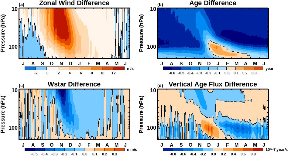
Figure 1. (a) Seasonal evolution of differences (1996-2010 minus 1960-1974) in zonal mean zonal wind at 60°S. The increase of zonal wind in late spring/summer indicates a delayed breakup of the Antarctic polar vortex. (b) Same as (a) but for Antarctic mean age of air (averaged over 64°-90°S). The increase of mean age in the summer lower stratosphere is partly due to the delayed breakup of the Antarctic polar vortex. (c) Same as (a) but for Antarctic vertical residual velocity (averaged over 64°-90°S). The delayed breakup of the Antarctic polar vortex leads to an increase of downwelling. (d) Same as (a) but for vertical flux of mean age (averaged over 64°-90°S). The enhanced downward transport of old air into the lower stratosphere also contributes to the mean age increase.

Concerns for Ozone Layer Recovery

Reactive gases containing chlorine (Cl) and bromine (Br) destroy stratospheric ozone via catalytic cycles. Man-made ozone depleting substances (ODSs) are the main source of these gases but natural sources contribute too. Most ODSs have long residence times in the atmosphere, but very short-lived substances (VSLS) with lifetimes of less than half a year also contribute to stratospheric ozone loss. The Montreal Protocol (MP) and its amendments have successfully regulated most man-made long-lived ODSs, leading to decline in atmospheric chlorine and bromine levels since the mid-1990s. Chlorine and bromine are expected to return to their 1980 level by ~2050, and stratospheric ozone will to return by ~2060. Concerns are now emerging that non-compliance with the Montreal Protocol, climate change, and rising VSLS emissions will delay the recovery of the ozone layer.

Recent research has highlighted the rapid growing atmospheric levels of a chlorinated VSLS called dichloromethane (CH2Cl2 or DCM). DCM is primarily man-made, but because of its short lifetime it is not controlled by the MP. It has widespread industrial uses and can be used as a substitute for the now-regulated ODSs. If the recently observed high DCM growth rate continues it could slow down stratospheric ozone recovery. However, it is unlikely that the current high growth rate will continue for decades because it would exceed the current global production capacity. But even if it did, the impact of DCM on ozone would still be small because DCM would only contribute about 4% to the expected stratospheric chlorine and bromine budget in 2050, resulting in a 2% loss of Antarctic column ozone.

Incomplete compliance with the MP is of greater concern for stratospheric ozone recovery than DCM. Currently carbon tetrachloride (CCl4), a potent ODS regulated by the MP, has ~35 Gg/yr of unaccounted for emissions. Because its lifetime is about 33 years, its emissions increases will have long and lingering impacts on stratospheric ozone.

The biggest uncertainty in stratospheric ozone recovery comes from human-induced perturbations to climate that may increase natural emissions of methyl bromide, methyl chlorine, and VSLS gases. If climate change increases atmospheric concentrations of these gases by 30%, which may happen by the end of the century, the resulting impact on the stratospheric ozone would be bigger than that from the man-made ODSs. Improved compliance and monitoring of regulated ODSs and limiting climate change are crucial to countering these threats.

Citation:
Liang, Q., S. E. Strahan, and E. L. Fleming, 2017. Concerns for ozone recovery. Science, 358 (6368): 1257-1258, DOI: 10.1126/science.aaq0145.

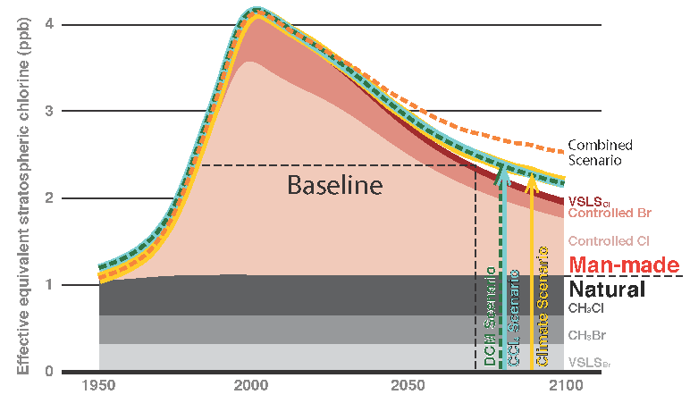
Figure 1. Estimated equivalent effective stratospheric chlorine (EESC) in the Antarctic lower stratosphere between 1950-2100. The baseline estimate assumes atmospheric DCM concentration remains at the present level, zero CCl4 emissions from present to 2100, and zero climate-induced changes in the natural emissions. Four additional EESC scenarios are also shown, a DCM scenario with ~2 ppt/yr increase into 2100 (dark green dashed line), a CCl4 scenario with a continued 35 Gg/yr emissions (teal solid line), a climate scenario with 30% increase in natural emissions between 1950 and 2100 (yellow solid line), a DCM+CCl4+Climate scenario (orange dashed line) showing the summed impact of all three. The vertical lines indicate the expected recovery year for the Antarctic ozone to return to the 1980 level for each scenario.

The role of sulfur dioxide in stratospheric aerosol formation evaluated by using in situ measurements in the tropical lower stratosphere

There has recently been a renewed interest in stratospheric aerosols-tiny droplets and particles suspended in the atmosphere at altitudes above where clouds form and where jet aircraft fly. In part this interest stems from a recognition that these particles, which primarily cool Earth's surface by reflecting incoming sunlight, can play a role in offsetting some of the warming caused by increased greenhouse gases, and there is the possibility that changes in manmade emissions from the surface and recent volcanic activity can be changing the amount and composition of these particles. Also, new satellite instruments are making measurements of these particles that are being used to inform models of Earth's climate system. Still, there are many things not well known, such as the sizes, composition, evolution, and sources of these particles.

Our study addresses the question of source mechanisms. The prevailing idea has been that inputs of sulfur dioxide gas, emitted from power plants and volcanic sources and later converted to particles, is the dominant source of stratospheric aerosols. During the autumn of 2015 a new instrument was flown onboard NASA's WB-57 high-flying aircraft, flying out of Houston, Texas, and over the US, Mexico, and the Gulf of Mexico at altitudes of nearly 60,000 feet (typical jet airliners fly at about 35,000 feet). The instrument flown used a laser-induced fluorescence technique that measured the concentration of sulfur dioxide. The measurements were compared to results from two Earth system models, the NASA GEOS-5 and NCAR WACCM models, that simulate transport and chemical composition of the atmosphere, and were also compared to measurements from two different satellite instruments, called MIPAS and ACE (Figure 1). The aircraft measurements agreed well with both of the models and the ACE measurements, but showed that the actual sulfur dioxide concentration in the lower stratosphere was much less than the MIPAS measurements showed. This is an important result, because MIPAS has been used to constrain global climate model simulations of the lower stratosphere. The lower sulfur dioxide concentrations obtained in the WB-57 aircraft flights have further been used to estimate the total flux of sulfur that enters the lower stratosphere, finding an amount that is only about 2% as large as the high end of the range of values reported in modeling studies. This creates a science puzzle on the origin and fate of these aerosols. Possible explanations are that directly injected particles from organic sources and other sulfur containing gases would explain the observed burden of sulfur in the stratosphere, or else that the aerosol losses from the stratosphere have been greatly overestimated in current models.

Citation:
Rollins, A.W., T.D. Thornberry, L.A. Watts, P. Yu, K.H. Rosenlof, M. Mills, E. Baumann, F.R. Giorgetta, T.V. Bui, M. Höpfner, K.A. Walker, C. Boone, P.F. Bernath, P.R. Colarco, P.A. Newman, D.W. Fahey, and R.S. Gao, 2017. The Role of Sulfur Dioxide in Stratospheric Aerosol Formation Evaluated Using In-Situ Measurements in the Tropical Lower Stratosphere. Geophys. Res. Lett., 44, 4280-4286, DOI: 10.1002/2017GL072754.

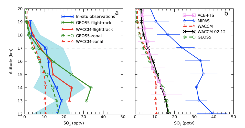
Figure 1. Measured and modeled sulfur dioxide (SO2) profiles in the tropical (10-25°N) upper troposphere/lower stratosphere (UT/LS). (a) The blue line and the shaded region show the aircraft in situ measurement median and interquartile range. WACCM and GEOS-5 have been adjusted upward by 1 km to match the aircraft ozone and thermal tropopause level. Two profiles each are shown for WACCM and GEOS-5: one for the zonal mean for 2015 (dashed lines) and another showing data sampled from the models along the flight track locations/times (solid lines). (b) Satellite ACE-FTS median and interquartile range (2004-2010) and MIPAS median and interquartile range of monthly means (2002-2012). Data during periods affected by major volcanic events were omitted from the ACE- FTS and MIPAS data. WACCM and GEOS-5 profiles are the same zonal mean profiles shown in Figure 1a. WACCM 02-12 profile (black) shows the mean profile obtained by sampling the WACCM run during the 2002- 2012 MIPAS period from the same times and locations as the MIPAS data that are averaged to derive the blue MIPAS profile.

A Model and Satellite-Based Analysis of the Tropospheric Ozone Distribution in Clear Versus Convectively Cloudy Conditions

Deep convection impacts the tropospheric ozone distribution by vertically redistributing ozone and its precursors. Surface air typically has lower ozone concentrations than upper tropospheric air; so convective lifting brings low ozone concentrations to the upper troposphere. On the other hand, over polluted regions it can also bring up pollutants that lead to ozone formation. Clouds also impact ozone chemistry and alter the amount of solar radiation available for ozone production.

Ziemke et al. [2009; 2017] developed a method for calculating the ozone concentration inside tropical deep convective clouds using data from the OMI and MLS instruments. This data is valuable for testing how well global chemistry climate models (CCMs) simulate the impact of clouds and convection on ozone. However, comparing CCMs to this data is not straightforward because each model grid box often contains both clear and cloudy regions, plus the GCM meteorology does not exactly match the observed for a specific day. We develop a method for comparing GEOSCCM ozone to the OMI/MLS in-cloud ozone data by defining the model output as "cloudy" for a given day and location if the daily mean cloud fraction is greater than 40%. Using this method, we find good agreement between the simulated in-cloud ozone and the observations. We use the model to quantify the effects of large-scale transport, convection, and chemistry on ozone in the middle troposphere. We find that convection acts to reduce ozone at 400 hPa over most of the tropics, but over highly polluted regions of South and East Asia, convection increases 400 hPa ozone. This study provides a new method for testing how well CCMs simulate the relationships between clouds, convection, and ozone.

Citation:
Strode, S. A., Douglass, A. R., Ziemke, J. R., Manyin, M., Nielsen, J. E., & Oman, L. D., 2017. A model and satellite-based analysis of the tropospheric ozone distribution in clear versus convectively cloudy conditions., J. Geophys. Res.: Atmos, 122, 11,948-11,960. DOI: 10.1002/2017JD027015.

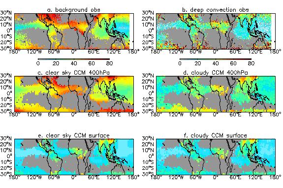
Figure 1. Observations based on the OMI and MLS instruments (top) show pronounced differences in tropical ozone concentrations on clear (left) versus cloudy (right) days. The GEOSCCM 400 hPa ozone (middle panels) reproduces many of these features. In contrast, the simulated surface ozone (bottom) shows little difference between clear and cloudy days, highlighting the importance of convection for establishing the clear versus cloudy differences seen in the middle troposphere.

Roles of Different Forcing Agents in Global Stratospheric Temperature Changes

Since the beginning of the 1980s, global stratospheric temperatures have decreased at all altitudes. This cooling is not linear, and includes two abrupt descending steps in the early 1980s and mid-1990s, coincident with the major volcanic eruptions of El Chichón and Mount Pinatubo, respectively.

Using the NASA GEOS-5 Chemistry Climate Model, we isolate the role played by each major temperature forcing agent in causing the features observed in the time series of stratospheric temperature anomalies. These forcing agents are 1) greenhouse gases, 2) changing ozone depleting substances, 3) volcanic eruptions, and 4) the solar cycle. Greenhouse gases, while warming the troposphere, cool the stratosphere, and their effect on stratospheric temperature increases with their increasing concentrations. Increases in ozone depleting substances also cause a cooling of the stratosphere, due to the subsequent decrease in ozone. But ozone depleting substances have been decreasing since the mid-1990s thanks to the limitations imposed by the Montreal Protocol. Our study shows that this decrease in ozone depleting substances, and, therefore, of the associated ozone depletion, caused the stall in the cooling of the lower stratosphere.

Sporadic volcanic events and the solar cycle have a distinct signature in the time series of stratospheric temperature anomalies, but do not play a significant role in the long-term trends from 1979 to 2015, Several factors combine to produce the step-like behavior in the stratospheric temperatures: in the lower stratosphere, the flattening starting in the mid-1990s is due to the decrease in ozone-depleting substances; Mount Pinatubo and the solar cycle cause the abrupt steps through the aerosol-associated warming and the volcanically induced ozone depletion. In the middle and upper stratosphere, changes in solar irradiance are largely responsible for the step-like behavior of global temperature anomalies, together with volcanically induced ozone depletion and water vapor increases in the post-Pinatubo years.

Citation:
Aquila, V., W. H. Swartz, D. W. Waugh, P. R. Colarco, S. Pawson, L. M. Polvani, R. S. Stolarski, 2016. Isolating the roles of different forcing agents in global stratospheric temperature changes using model integrations with incrementally added single forcings, J. Geophys. Res., in press, DOI: 10.1002/2015JD023841.

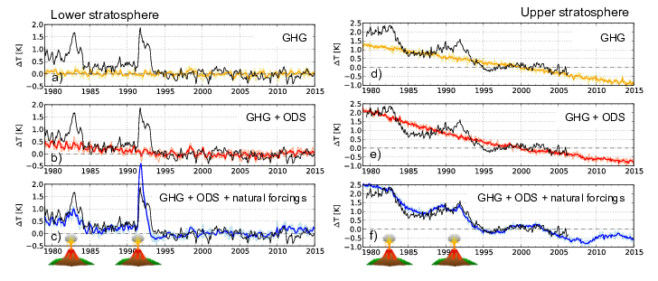
Figure 1. Changes in global temperature anomalies in the lower (left) and upper (right) stratosphere in observations (black) and in the model simulations performed with the NASA GEOS-5 chemistry climate model (GEOSCCM) by incrementally adding the effects of (a, d) increasing greenhouse gases, (b, e) changing ozone depleting substances, and (c, f) volcanic eruptions and the solar cycle on the climate system.

Transport of ice into the stratosphere and the humidification of the stratosphere over the 21st century

Models project that as the climate warms the amount of water vapor entering the stratosphere will increase. While the end result appears to be a robust response from climate models the exact mechanism has not been examined in detail. Changes in water vapor in the lower stratosphere can have important feedbacks to the surface climate response to warming, so it is critical to understand its causes.

A new study by scientists at Texas A&M University, NASA's Goddard Space Flight Center (GSFC), and NOAA's Earth System Research Laboratory used comprehensive chemistry-climate models (CCM) along with simplified trajectory models to quantify the causes of increased water vapor over the 21st century. Using this unique combination of models allows the mechanism behind the water vapor changes to be quantified. It showed the current thinking that water vapor responds to temperature changes in the tropical tropopause layer (TTL) is not entirely correct and that a significant portion comes from the lofting and re-evaporation of convective ice above the TTL.

This work improves our understanding of what drives stratospheric water vapor to change over this century. In addition it helps to refine what observations are necessary to understand this behavior in the real atmosphere. This study is part of a larger chemistry climate project at GSFC using computer simulations of our atmosphere to improve our knowledge of Earth's climate system.

Citation:
Dessler, A. E., H. Ye, T. Wang, M. R. Schoeberl, L. D. Oman, A. R. Douglass, A. H. Butler, K. H. Rosenlof, S. M. Davis, and R. W. Portmann, 2016. Transport of ice into the stratosphere and the humidification of the stratosphere over the 21st century. Geophys. Res. Lett., 43, DOI: 10.1002/2016GL067991.

Description and Validation of CH4-CO-OH (ECCOHv1.01) chemistry module for 3-D model applications

In this paper, we described and validated a new computationally Efficient CH4-CO-OH chemistry module (ECCOH) that allows for the simulation of the methane, carbon monoxide and hydroxyl radical (CH4-CO-OH) system, within a chemistry climate model, carbon cycle model, or earth system model. The computational efficiency of the module allows many multi-decadal sensitivity simulations of the CH4-CO-OH system, which primarily determines the global atmospheric oxidizing capacity. This capability is important for capturing the nonlinear feedbacks of the CH4-CO-OH system and understanding the perturbations to methane, CO and OH and the concomitant impacts on climate. We implemented the ECCOH chemistry module into the NASA GEOS-5 Atmospheric Global Circulation Model (AGCM), performed multiple sensitivity simulations of the CH4-CO-OH system over two decades, and evaluated the model output with surface and satellite datasets of methane and CO. The favorable comparison of output from the ECCOH chemistry module (as configured in the GEOS-5 AGCM) with observations demonstrates the fidelity of the module for use in scientific research. This work has been developed entirely at GSFC.

Citation:
Elshorbany, Y. F., B. N. Duncan, S. A. Strode, J. S. Wang, and J. Kouatchou, 2016. The description and validation of a computationally-Efficient CH4-CO-OH (ECCOHv1.01) chemistry module for 3-D model applications. Geosci. Model Dev., 9, 799-822, DOI: 10.5194/gmd-9-799-2016.

Interpreting Space-based Trends in Carbon Monoxide with Multiple Models

Concentrations of the pollutant carbon monoxide (CO) vary over time due to trends in anthropogenic emissions as well as year-to-year variability in biomass burning. Worden et al. [2013] found significant negative trends in CO observations from MOPITT over the eastern United States, Europe, and eastern China. While negative trends over the United States and Europe are consistent with decreasing emissions due to pollution control measures, the negative trend over eastern China is unexpected based on the positive trends in emissions from this region found in several emission inventories. In this study, we use a suite of global model simulations to interpret the observed trends. We find that simulations using time-dependent emissions reproduce the observed trends over the eastern United States and Europe, suggesting that the time-dependent emission inventory is reasonable over these regions. The simulations produce a positive trend over eastern China, in contrast with the observed trend. This discrepancy between the simulated and observed trends likely indicates that the assumed emission trend over China is too positive. However, several other factors contribute to the discrepancy, including large variability in the simulated ozone column, which impacts the chemical loss of CO via reaction with OH.

Citation:
Strode, S.A., H.M. Worden, M. Damon, A.R. Douglass, B.N. Duncan, L.K. Emmons, J.F. Lamarque, M. Manyin, L.D. Oman, J.M. Rodriguez, S.E. Strahan, and S. Tilmes, 2016. Interpreting space-based trends in carbon monoxide with multiple models. Atmos. Chem. Phys., 16(11), 7285-7294, DOI: 10.5194/acp-16-7285-2016.

Antarctic and Southern Ocean climate change in the Goddard Earth Observing System (GEOS-5)

Antarctic ozone depletion plays an essential role in driving Southern Hemisphere climate change in the last 3-4 decades. The ozone hole cools the Antarctic stratosphere and increases the prevailing westerly winds, changing the large-scale circulation pattern in the troposphere and the Southern Ocean. Climate models use different approaches to represent stratospheric ozone climate forcing. The most realistic way is to calculate ozone interactively, which captures interactions between chemistry, radiation, and dynamics. However, many climate models, including those participating the IPCC report, simply prescribe monthly and zonally averaged ozone fields. These prescribed ozone fields have two major biases: they underestimate ozone hole and they lack ozone zonal variations. In this study we investigate the impacts of using interactive stratospheric chemistry instead of prescribed ozone on climate change simulations of the Antarctic and Southern Ocean.

We conducted two sets of 1960-2010 ensemble simulations with the coupled ocean version of the Goddard Earth Observing System Model version 5 (GEOS-5): one with interactive stratospheric chemistry and the other with prescribed ozone derived from the same interactive simulations. We have found that interactive chemistry has important effects on climate change not only in the Antarctic stratosphere, troposphere and surface, but also in the Southern Ocean and Antarctic sea ice. Interactive chemistry causes stronger Antarctic lower stratosphere cooling and stronger circumpolar westerly acceleration from the stratosphere to the surface during November-December-January. At the surface, the maximum westerly wind-stress trend in the interactive ozone simulations is twice as large in the prescribed ozone simulation. The stronger surface wind-stress trends cause larger increases of the Southern Ocean overturning circulation, leading to year-round stronger warming near the surface and enhanced Antarctic sea ice decrease. These results highlight the importance of correctly representing ozone hole forcing in order to fully capture its effects on climate change.

Citation:
Li. F., Y. V. Vikhliaev, P. A. Newman, S. Pawson, J. Perlwitz, D. W. Waugh, and A. R. Douglass, 2016. Impacts of interactive stratospheric chemistry on Antarctic and Southern Ocean climate change in the Goddard Earth Observing System - Version 5 (GEOS-5). J. Climate, 29, DOI: 10.1175/JCLI-D-15-0572.1.

Is the Brewer-Dobson circulation increasing, or moving upward?

The circulation of air through the stratosphere impacts many important quantities, including trace gas species like ozone and water vapor. By observing the distribution of these species, this circulation, now called the Brewer Dobson Circulation (BDC), was originally theorized. Any future changes in the strength of this circulation can cause significant changes to the distribution of these and other trace gas species.

A new collaborative study by scientists at a number of Universities, Research Institutes, and NASA's Goddard Space Flight Center (GSFC) used chemistry-climate models (CCM) to understand how the BDC is projected to change. Using a large number of simulations from several different CCM's, the causes of changes in the BDC could be isolated. CCM's showed that most of the increase in the lower stratospheric BDC is occurring because of a warming troposphere and rising tropopause, causing the circulation to move upward in the atmosphere.

This work provides a new view on how the BDC is expected to change in the future and will allow us to make more careful targeted observations of the effect. Using simulations from a variety of CCM's helps to understand the robustness of the model response. This study is part of a larger chemistry climate modeling initiative (CCMI) project using computer simulations of our atmosphere to improve our knowledge of Earth's climate system.

Citation:
Oberländer-Hayn, S., E. P. Gerber, J. Abalichin, H. Akiyoshi, A. Kerschbaumer, A. Kubin, M. Kunze, U. Langematz, S. Meul, M. Michou, O. Morganstern, and L. D. Oman, 2016. Is the Brewer-Dobson circulation increasing or moving upward? Geophys. Res. Lett., 43, DOI: 10.1002/2015GL067545.

Effect of Recent Sea Surface Temperature Trends on the Arctic Stratospheric Vortex

Sea Surface Temperature (SST) anomalies are a dominant driver of atmospheric variability on a variety of timescales. However, depending on the location, sign, and magnitude of these SST anomalies the resulting impacts can differ. The difference in SSTs can impact atmospheric dynamics not only in the troposphere, the lowest layer of our atmosphere, but also the layer above it, the stratosphere.

A new study by scientists at Hebrew University and NASA's Goddard Space Flight Center (GSFC) used a chemistry-climate model (CCM) to understand how recent SST trends have influence the Arctic stratospheric vortex. Using a large number of targeted simulations with the Goddard Earth Observing System (GEOS) version 5 CCM, the impact of SST changes on the Arctic stratospheric vortex could be isolated. GEOSCCM showed that the warming of the Indian Ocean, North Pacific, and North Atlantic along with cooling of the tropical Pacific have strongly contributed to recent polar stratospheric cooling in late winter and early spring. These changes in the Arctic vortex can be understood by examining the tropospheric height and heat flux anomalies generated by the SST anomalies.

This work improves our understanding of how sea surface temperatures impact recent changes in the Arctic stratospheric vortex. Using targeted simulations from GEOSCCM the impact on stratospheric dynamics from variations in SST continue to be unraveled. This study is part of a larger chemistry climate project at GSFC using computer simulations of our atmosphere to improve our knowledge of Earth's climate system.

Citation:
Garfinkel, C. I., M. M. Hurwitz, and L. D. Oman, 2015. Effect of recent sea surface temperature trends on the Arctic stratospheric vortex. J. Geophys. Res. Atmos., 120, 5404-5416, DOI: 10.1002/2015JD023284.

Air-Mass Origin in the Arctic. Part I: Seasonality

The Arctic is warming faster than any other region on Earth. Part of this accelerated warming is related to processes that occur very far away. Most noticeably, studies have shown that black carbon (i.e. soot) emissions from midlatitude power plants travel all the way to the Arctic and warm the surface by reducing the reflectivity of ice and snow. To understand climate, therefore, we need to understand the distant origins of Arctic air and pollution.

Scientists use models and observations to understand the meteorological and physical conditions that enhance pollution transport to the Arctic. One common approach is to compare observations and models during individual transport events -- for example, the daily evolution of a single weather system as it sweeps Asian pollution poleward to higher latitudes. This approach allows models to be validated in detail with observations sampled by aircraft and balloon instruments. However, because of the specific conditions of single transport events, this approach only anecdotally connects midlatitude emissions to the Arctic. It is the accumulated transport over many events and large spatial scales that ultimately determines climate and its long-term changes.

Pollution transport is often studied in the context of a single (or a few) chemical species, all of which feature different chemical properties and emission patterns. As it stands, therefore, there is a gap in our scientific understanding of pollution transport that makes it hard to quantitatively link circulation patterns like the jet stream to Arctic pollution levels. This is important for climate studies, however -- in particular for understanding how the Arctic will respond to changes in winds, temperature, and various circulation patterns resulting from global warming.

In this study we use a climate model to show that more than 60% of boundary layer air in the Arctic is of midlatitude origin. In addition, there are strong seasonal variations in the midlatitude boundary layer regions that supply air to the Arctic - the oceans dominate in winter and the continents in summer. Furthermore, all origin regions are not created equal, as Asia supplies more than 40% of all midlatitude boundary layer air to the Arctic during summer. This is especially concerning since black carbon emissions over Asia have been increasing over recent decades, with little sign of decreasing.

These results have important implications for understanding current and future Arctic climate in the context of the large-scale circulation. As the climate warms circulation patterns over midlatitudes will change. Our results suggest that these changes -- specifically over the East Pacific and Asia -- may contribute to changes in Arctic pollution, irrespective of whether or not pollutant emissions change.

Citation:
Orbe, C., Newman, P. A., Waugh, D. W., Holzer, M., Oman, L. D., Li, F., and Polvani, L. M., 2015. Air-Mass Origin in the Arctic. Part I: Seasonality. Journal of Climate,28, 4997-5014, DOI: http://dx.doi.org/10.1175/JCLI-D-14-00720.1.

Air-mass Origin in the Tropical Lower Stratosphere

Pollution that is emitted at the Earth's surface and enters the stratosphere can impact stratospheric ozone, water vapor and aerosols, which control key aspects of climate. For example, recent studies have shown that short-lived trace gases emitted over the oceans played an important role in 20th century stratospheric ozone depletion. Other studies have shown that aerosols released from volcanoes and produced in power plants contribute to the seasonal changes and, possibly, long-term trends of the stratospheric aerosol layer, which is important for maintaining the Earth's balance of incoming and outgoing solar radiation.

Short-lived trace gases and aerosols can impact stratospheric climate provided there are efficient and fast transport paths that connect the stratosphere to the Earth's surface. While most transport to the stratosphere happens over the tropics, recent studies have shown that the Asian monsoon circulation also efficiently transports water vapor and pollution to the extratropical lower stratosphere.

Satellite observations and numerical models confirm that traces of the Asian monsoon appear among a wide range of trace species. These signatures reflect, however, not only the underlying transport by the circulation but also the emissions patterns and chemical interactions specific to each species. This lack of "transport-only" information in turn makes it hard to unambiguously link the large-scale circulation features of the Asian monsoon to upper tropospheric and lower stratospheric composition.

In addition, modeling studies have compared observations with models during individual monsoon periods, which allows models to be validated in detail with observations sampled by aircraft and balloon instruments. Because of the specific conditions of single transport events, however, this approach only anecdotally connects pollution emitted over Asia to the lower stratosphere. And yet, it is the accumulated transport over many events and large spatial scales that ultimately determines climate and its long-term changes. Few transport measures and model-based climatologies, therefore, have made it difficult to tackle climate problems regarding the influence of the monsoon on the stratosphere.

In this study we use a climate model to look at the underlying long-term transport that links the Earth's surface to the stratosphere. We show that nearly 20% of air in the tropical lower stratosphere originates in the Asian boundary layer, compared to negligible amounts from North America and Europe. This implies that Asian emissions are much more efficient at reaching the stratosphere than emissions from other populated regions. This result is interesting given that Asian emissions of black carbon (i.e. soot) have been increasing in recent decades and show little signs of decreasing.

Overall, our study shows that transport from the Asian boundary layer to the lower stratosphere is not only anecdotally important but also a key part of the long-term climate properties of the lower stratosphere. We also show that the transport paths that connect the Asian surface to the stratosphere involve the confinement of air inside of the monsoon anticyclone and its penetration into the stratosphere outside of the deep tropics.

By focusing on origin in the planetary boundary layer we provide a way to link the monsoon circulation to the lower stratosphere using a framework that can be applied to any climate model to understand not only present-day but future pollution in the stratosphere. Our study strongly suggests that changes in the monsoon circulation over Asia need to be considered when interpreting trace species budgets in the lower stratosphere and future responses to global climate change.

Citation:
Orbe, C., Waugh, D. W., and Newman, P. A., 2015. Air-mass origin in the tropical lower stratosphere: The influence of Asian boundary layer air. Geophys. Res. Lett., 42, 4240-4248, DOI: 10.1002/2015GL063937.

The Atmospheric Chemistry of Nitrous Oxide and its Changing Lifetime

Nitrous oxide (N2O) is an important gas that has both natural and humankind sources. N2O impacts the chemical composition of the Earth's atmosphere, including the ozone layer, and also traps infrared radiation that leads to global warming. The destruction in the atmosphere of nitrous oxide occurs either by chemical reaction or by ultraviolet (UV) light from the sun. The rate at which N2O is destroyed can be estimated by laboratory measurements. This rate of destruction can then be used with computer models of the atmosphere and satellite measurements of the N2O concentration to determine how long a molecule of N2O resides in the atmosphere prior to its destruction. This residence time is referred to as the lifetime, and is important in determining the length of time over which a molecule of N2O will have a significant impact on the ozone layer and on global warming.

This paper provides a detailed analysis of the determination of the N2O lifetime using satellite data together with laboratory measurements of the rate of N2O destruction and several computer models of the global atmosphere. The result is a lifetime of 116 years, giving N2O a long residence time in the atmosphere. The lifetime determination also has various sources of error, referred to as uncertainty, due to limitations and inaccuracies in the satellite data and laboratory measurements, and the range of results obtained by the different computer models. After accounting for all the sources of error, the N2O lifetime is expected to be between 107 and125 years. This study also shows that another important factor in determining the lifetime is the amount of N2O present in the atmosphere. This effect, known as feedback, will reduce the N2O lifetime in the future as atmospheric N2O concentrations are projected to increase due to human activity. The results from this study will ultimately increase our confidence in quantifying the past and future impacts on ozone and global warming from N2O.

Citation:
Prather M. J., Hsu J., DeLuca N. M., Jackman C. H., Oman L. D., Douglass A. R., Fleming E. L., Strahan S. E., Steenrod S. D., Søvde O. A., Isaksen I. S. A., Froidevaux L., and Funke B.,2015. Measuring and modeling the lifetime of nitrous oxide including its variability. J. Geophys. Res. Atmos., 120, 5693-5705, DOI: 10.1002/2015JD023267.

Use of North American and European air quality networks to evaluate global chemistry-climate modeling of surface ozone

We test global chemistry--climate models in their ability to simulate present-day surface ozone. Models are tested against observed hourly ozone from 4217 stations in North America and Europe that are averaged over 1°x1° grid cells. Using novel metrics, we find most models match the shape but not the amplitude of regional summertime diurnal and annual cycles and match the pattern but not the magnitude of summer ozone enhancement. Most also match the observed distribution of extreme episode sizes.

Citation:
Schnell, J. L., M. J. Prather, B. Josse, V. Naik, L. W. Horowitz, P. Cameron-Smith, D. Bergmann, G. Zeng, D. A. Plummer, K. Sudo, T. Nagashima, D. T. Shindell, G. S. Faluvegi, and S. A. Strode, 2015. Use of North American and European air quality networks to evaluate global chemistry-climate modeling of surface ozone. Atmos. Chem. Phys., 15: 10581-10596, DOI: 10.5194/acp-15-10581-2015.

Implications of CO bias in Chemistry-Climate Models

Carbon monoxide (CO) plays an important role in tropospheric chemistry. It is the primary sink of the hydroxyl radical (OH), an important atmospheric oxidant, and thus impacts how quickly atmospheric constituents such as methane (CH4) are oxidized. Chemistry climate models (CCMs) often have a low bias in CO in the high northern latitudes. This underestimate of CO could lead to an overestimate of OH and underestimate of the methane lifetime. On the other hand, it is possible that other factors drive a bias in simulated OH, which in turn causes a bias in CO. Determining the cause of CO bias is important for improving model simulations of OH and the lifetime of CH4, since CH4 is a potent greenhouse gas. We examined possible causes of the low bias in northern latitude CO in the GEOS-5 Chemistry Climate Model (GEOSCCM). We used tracers of CO from specific regions and sources to examine the sensitivity of the global mean CO and the interhemispheric gradient of CO to emissions from different regions. We also conducted experiments altering OH concentrations globally or just in the northern hemisphere, and found that reducing OH by twenty percent in the northern hemisphere improved our simulation of CO. We next conducted simulations using a parameterization for OH concentrations to test the sensitivity of OH to known model biases in other constituents. We adjusted the inputs to the parameterization such as ozone and water vapor to match the values seen in satellite data or the Modern Era-Retrospective Analysis for Research and Applications (MERRA). We found that none of the individual adjustments leads to a large enough decrease in OH to explain the CO bias. However, all of the adjustments together lead to an increase in the simulated methane lifetime that agrees well with observation based estimates.

Citation:
Strode, S.A., B.N. Duncan, E.A. Yegorova, J. Kouatchou, J.R. Ziemke, and A.R. Douglass, 2015. Implications of carbon monoxide bias for methane lifetime and atmospheric composition in chemistry climate models. Atmos. Chem. Phys., 15, 11789-11805, DOI: 10.5194/acp-15-11789-2015.

Effects of Geoengineering on the Quasi-biennial Oscillation

Geoengineering is the deliberate modification of the Earth's system in order to counteract global warming due to increasing greenhouse gases. One proposed geoengineering method involves the injection of sulfate aerosol in the stratosphere, and aims to reproduce the cooling that have been observed after major volcanic eruptions. A side effect of the injection of these stratospheric aerosol is the warming of the stratosphere, and the subsequent perturbation of the stratospheric dynamics.

GEOSCCM model simulations showed that a geoengineering stratospheric injection of aerosol could dramatically perturb the periodicity of the quasi-biennial oscillation (QBO). The QBO is the oscillation of zonally symmetric easterly and westerly winds in the tropical stratosphere with an a verage period of about 28 months. The vertical descending of the shear of the QBO is linked to the mean tropical upwelling of the Brewer Dobson circulation. Geoengineering simulations performed with GEOSCCM show that the phase of easterly shear is prolonged with respect to the control case, with a period that becomes longer with increasing stratospheric burdens of aerosols. This is due to the absorption of IR radiation from the aerosol in the tropical stratosphere, which increases the vertical upwelling and perturbs the vertical transport of momentum. If the burden of geoengineering aerosol exceed a certain threshold, the oscillation is interrupted and the stratosphere is in a state of perpetual westerlies. No previous study has investigated the effect of geoengineering on the QBO. Even if the QBO is limited to the tropics, its phase affects the stratospheric transport to the extratropics and the strength of the polar vortex. These results show that SRM might have an indirect impact on the mixing between tropics and extratropics, and on ozone depletion via changes in the strength of the polar vortex.

Citation:
Aquila, V., C. I. Garfinkel, P. A. Newman, L. D. Oman, and D. W. Waugh, 2014. Modifications of the quasi-biennial oscillation by a geoengineering perturbation of the stratospheric aerosol layer. Geophys. Res. Lett., 41, 1738-1744, DOI: 10.1002/2013GL058818.

Geoengineering QBO Figure 1

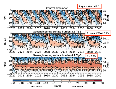
Figure 1. Here we show the simulated vertical profiles of equatorial stratospheric zonal winds from the start of the geoengineering injection in January 2020 to December 2040. Red shaded areas mark westerly (or eastward blowing) winds, blue shaded areas easterly (or westward blowing) winds. The upper panel shows the control simulation - with no sulfate aerosol. The middle and lower panels show the simulations with geoengineering sulfate burdens of 3.1 Tg-Sulfate (middle) and 4.7 Tg-Sulfate (bottom).

Improvements in Modeling Ozone and Application to a New Scenario

The evolution and recovery of Earth's ozone layer is an important science question that relies on satellite measurements and chemistry-climate model projections. Ozone is a very important atmospheric gas that absorbs damaging ultraviolet radiation, so changes in the total amount above us can have significant consequences for our biosphere. Chemistry-climate models are crucially important to projecting the future evolution of ozone and to understand the factors that drive this change.

A new study by scientists at NASA's Goddard Space Flight Center (GSFC) documented and demonstrated improvements to the Goddard Earth Observing System Chemistry-Climate Model (GEOSCCM) specifically focusing on total column ozone. They found that by including more processes known from observations model biases could be significantly reduced. These processes include: the Quasi-Biennial Oscillation of tropical stratospheric winds, variability of observed stratospheric sulfate aerosol, and improvements in the day/night transition in the chemical mechanism among others. These changes were compared to satellite and ground-based observation which showed a much improved GEOSCCM. This new version was then used to simulate future ozone with a new scenario of ozone depleting substances to support the upcoming World Meteorological Organization's (WMO) scientific assessment of ozone report.

The improvements to GEOSCCM have relevance to many other important trace gas species, which will continue to be explored. Future work will use more NASA satellite measurements to continue to guide model development in more faithfully reproducing our complex climate system. This work is part of a larger chemistry-climate project at GSFC with the ultimate goal of using computer modeling and observations to improve our knowledge of Earth's climate system.

Citation:
Oman, L. D., and A. R. Douglass, 2014. Improvements in total column ozone in GEOSCCM and comparisons with a new ozone-depleting substances scenario. J. Geophys. Res. Atmos., 119, 5613-5624, DOI: 10.1002/2014JD021590.

New Scenario Figure 1

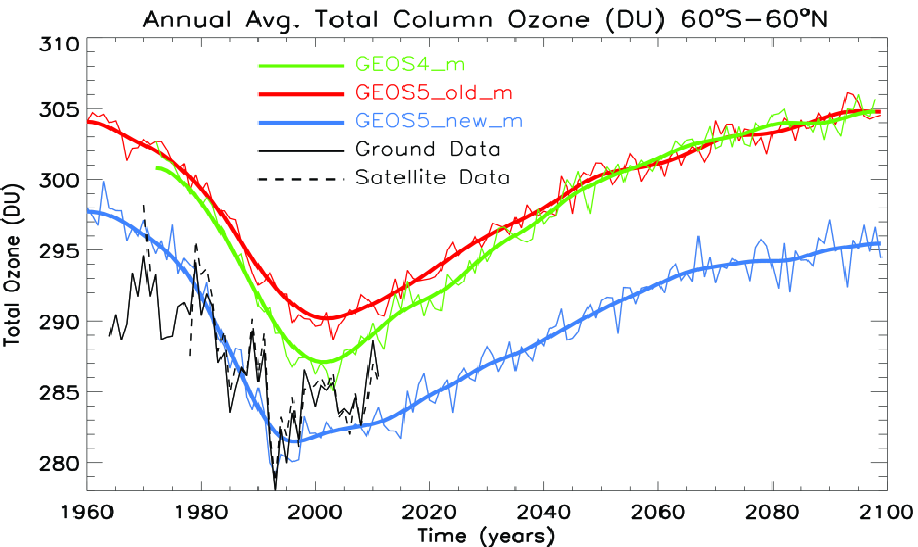
Figure 1. Annual average quasi-global (60 degrees S - 60 degrees N) total column ozone (DU) for GEOS4 (green curve), GEOS5_old (red curve),GEOS5_new (light blue curve), ground-based measurements (black solid curve), and satellite-based measurements (black dashed curve). GEOS4 simulation is from 1971-2098, the GEOS5 simulations are from 1960-2099 and the ground-based observations are from 1964-2011. The thick lines are output smoothed to remove interannual variability.

Effects of Geoengineering on Stratospheric Ozone

Geoengineering is the deliberate, large-scale modification of the Earth's climate system in order to counteract the warming effects of increasing greenhouse gases. Some proposed geoengineering methods, referred to as solar radiation management (SRM), aim to alleviate the effects of climate change by reducing the solar radiation reaching the Earth surface. The Geoengineering Model Intercomparison Project (GeoMIP) is an international collaboration with the goal of understanding the effects of geoengineering solar radiation management through climate simulations performed with different global climate models.

One specific solar radiation management method mimics the cooling effect of large volcanic eruptions by prescribing the artificial injection of sulfate aerosol particles in the stratosphere. However, observations of post-eruption periods showed that stratospheric concentrations of ozone tend to decrease because of the increased levels of stratospheric aerosol.

Model simulations by GEOSCCM and other GeoMIP participating models show that the geoengineering injection of stratospheric aerosol would lead to a net decrease of global ozone via several mechanisms. First, the presence of the aerosol modifies the radiation penetrating in the stratosphere and, subsequently, the photolysis processes involving ozone. Second, the absorption of longwave radiation from the aerosol warms the lower stratosphere, strengthening the tropical upwelling of ozone-poor air. Lastly, the geoengineering aerosol fosters the heterogeneous chemistry, via the increase of sulfate aerosol surface area density and polar stratospheric clouds.

Citation:
Pitari, G., V. Aquila, B. Kravitz, A. Robock, S. Watanabe, I. Cionni, N. De Luca, G. Di Genova, E. Mancini, and S. Tilmes, 2014. Stratospheric ozone response to sulfate geoengineering: Results from the Geoengineering Model Intercomparison Project (GeoMIP). J. Geophys. Res. Atmos., 119, 2629-2653, DOI: 10.1002/2013JD020566.

Seasonal variation of ozone in the tropical lower stratosphere: Southern tropics are different from Northern tropics

The circulation of the stratosphere has been long known to play an important role in the seasonal cycle of ozone and other trace gas constituents. Typically the seasonal cycle of the tropics has been treated as a whole, however, significant differences occur between the Northern Hemisphere and Southern Hemisphere tropics. Examining trace gas constituents such as ozone from satellite measurements illuminate the underlying transport and contain information on circulation and mixing properties in different regions.

A new study by scientists at Johns Hopkins University and NASA's Goddard Space Flight Center (GSFC) used measurements and models to show the importance of the stratospheric circulation and mixing on the seasonal cycle of tropical lower stratospheric ozone. The relative importance of circulation and mixing in each tropical hemisphere was determined using measurements from the Microwave Limb Sounder (MLS) onboard NASA's Aura satellite, Stratospheric Aerosol and Gas Experiment (SAGE) II, and ozonesondes. The stronger seasonal cycle in ozone in the northern tropics is related to the additive impact of upwelling and mixing occurring in phase, whereas in the southern tropics they are out of phase and diminish its magnitude. Using our new understanding of the roles of upwelling and mixing, a simple model of the tropical stratosphere reproduced the observed pattern of seasonal cycle magnitude and timing.

This work demonstrates the importance of the combined use of satellite, ground-based measurements, and models to understand variations in tropical lower stratospheric ozone and other trace gases. By closely examining the variations in the seasonal cycle within the tropics, this study goes beyond past work of treating the tropics as a whole. This research is part of a larger chemistry climate project at GSFC with the ultimate goal of using observations and computer simulations to improve our knowledge of Earth's climate system.

Citation:
Stolarski, R. S., D. W. Waugh, L. Wang, L. D. Oman, A. R. Douglass, and P. A. Newman, 2014. Seasonal variation of ozone in the tropical lower stratosphere: Southern tropics are different from Northern tropics. J. Geophys. Res., 119, 6196-6206, DOI: 10.1002/2013JD021294.

The Effect of Volcanic Eruptions on the Stratosphere

Volcanic eruptions inject in the atmosphere heavy ash particles and gaseous sulfur dioxide, which is transformed into sulfate aerosol particles through chemical reactions. While gravity rapidly removes the heavy particles from the atmosphere, sulfur dioxide and sulfate particles can be transported up to the stratosphere. At such altitudes, there are only few sinks for particles: the sulfate that reaches the stratosphere can remain for years and diffuse over the whole globe, inducing perturbation in the global climate. The major volcanic eruption of the 20th century was the one of Mt. Pinatubo, in the Philippines. Mt. Pinatubo injected in the atmosphere about 30 Tg of sulfate, which diffused over the whole globe within three weeks from the eruption.

Recent studies by scientists at the NASA Goddard Space Flight Center investigated the stratospheric effects of the Mt. Pinatubo eruption. These studies found that the transport of the volcanic aerosol was largely driven by the radiative interaction of the volcanic aerosol itself, which, absorbing largely longwave radiation, warmed the tropical stratosphere and increased the upwelling in the tropics. This induced a "self-lofting" of the volcanic cloud to up to 30 km altitudes. The increased upwelling in the tropics was followed by an increased downwelling in the extratropics.

Stratospheric volcanic aerosols enhances the heterogeneous chemical reaction that depletes NO2. This reactions usually leads to an increase of active chlorine, which results in a depletion of the ozone. After the eruption of Mt. Pinatubo observations at southern midlatitudes showed the expected depletion of the NO2 column, but, surprisingly, no depletion of the ozone column. The studies by NASA GSFC scientists show that the enhanced tropical upwelling and extratropical downwelling increased the ozone concentration at southern midlatitudes, masking the effects of the chemical depletion. The same ozone perturbation did not take place in the northern hemisphere because the Brewer-Dobson circulation during the season of the eruption is directed toward the southern hemisphere. Model experiments with a Mt. Pinatubo-like injection in January show a similar ozone increase in the northern hemisphere.

Citation 1:
Aquila, V., L.D. Oman, R.S. Stolarski, P. Colarco, and P. A. Newman, 2012. Dispersion of the volcanic sulfate cloud from a Mount Pinatubo-like eruption. J. Geophys. Res, 117, D06216, DOI: 10.1029/2011JD016968.

Citation 2:
Aquila, V., L. D. Oman, R. Stolarski, A. R. Douglass, P. A. Newman, 2013. The Response of Ozone and Nitrogen Dioxide to the Eruption of Mt. Pinatubo at Southern and Northern Midlatitudes. J. Atmos. Sci., 70, 894-900, DOI: 10.1175/JAS-D-12-0143.1.

Ozone Anomaly Figure 1

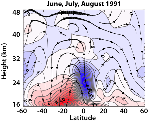
Figure 1. Vertical distribution of the ozone anomaly, in %. The streamlines show the enhanced tropical upwelling and extratropical downwelling due to the aerosol from the Mt. Pinatubo eruption. The enhanced circulation created a positive ozone anomaly at southern midlatitudes, which cancelled the ozone depletion due to chemistry on the volcanic aerosol.

Sensitivity of the atmospheric response to warm pool El Niño events to modeled SSTs and future climate forcings

Of the two types or "flavors" of El Niño observed in the past few decades, warm pool El Niño (WPEN) events are characterized by positive sea surface temperature anomalies in the central equatorial Pacific. Under present-day climate conditions, WPEN events disrupt the usual circulation pattern in the tropical atmosphere, generating large-scale atmospheric high and low-pressure wave patterns that propagate toward the poles and upward into the stratosphere. These patterns bring additional heat to the stratosphere, warming the Polar Regions in Northern Hemisphere autumn and winter. Thus, WPEN events explain some of the observed year-to-year variability of the polar stratosphere, in the season when polar ozone depletion occurs.

Since some studies suggest that WPEN events are becoming more frequent, the Goddard Earth Observing System Chemistry-Climate Model (GEOSCCM), a numerical climate model with interactive stratospheric chemistry, is used to investigate the response to WPEN events under projected late 21st century climate conditions. The future Arctic stratospheric response to WPEN events is qualitatively similar to that observed in recent decades. The response is weaker in late winter because the Northern Hemisphere wave patterns weaken slightly. In contrast, the Antarctic stratosphere does not respond to WPEN events in a future climate, reflecting a change in the structure of the wave patterns in the Southern Hemisphere sub-tropics. Simulated, late 21st century sea surface temperatures weaken the poleward wave pattern, while another wave pattern traveling eastward from Australia becomes dominant.

Citation:
Hurwitz, M. M., C. I. Garfinkel, P. A. Newman, and L. D. Oman, 2013. Sensitivity of the atmospheric response to warm pool El Niño events to modeled SSTs and future climate forcings. J. Geophys. Res. Atmos., 118, 13,371-13,382, DOI: 10.1002/2013JD021051.

Net influence of an internally generated quasi-biennial oscillation on modelled stratospheric climate and chemistry

The quasi-biennial oscillation (QBO) is an alternating pattern of easterly (westward) and westerly (eastward) winds in the equatorial lower stratosphere, approximately 20-30km above the Earth's surface. Each oscillation takes approximately 28 months. Observations show that the wintertime Arctic stratosphere is colder when the QBO is in its westerly phase, and that the phase of the QBO affects the transport of trace atmospheric constituents such as ozone.

The time-averaged impact of the easterly and westerly phases of the QBO on winds, temperature and ozone cannot be evaluated using atmospheric data because the QBO signal is intrinsic to the observational record. The GEOS chemistry-climate model can be used to estimate the net impact of the QBO by comparing 'QBO' and 'no QBO' simulations. Inclusion of the modeled QBO makes a significant difference to stratospheric temperature, circulation and sub-tropical mixing. The QBO enhances tropical and sub-tropical variability.

Inclusion of the QBO enhances polar stratospheric variability in winter. While tropical zonal winds in the 'no QBO' simulation are generally easterly, there is a relative increase in the mean tropical lower stratospheric winds in the 'QBO' simulation. Extra-tropical differences between the QBO and 'no QBO' simulations thus reflect a bias toward the westerly phase of the QBO: the polar stratosphere is colder, winds are stronger, and Arctic lower stratospheric ozone concentrations slightly decrease.

Citation:
Hurwitz, M. M., Oman, L. D., Newman, P. A., and Song, I.-S., 2013. Net influence of an internally generated quasi-biennial oscillation on modelled stratospheric climate and chemistry. Atmos. Chem. Phys., 13, 12187-12197, DOI: 10.5194/acp-13-12187-2013.

NASA's Aura Satellite Illuminates the Signature of ENSO in Lower Atmospheric Ozone

El Niño Southern Oscillation (ENSO) is the episodic warming or cooling of sea surface temperatures in the eastern and central equatorial Pacific and the dominant mode of interannual tropical variability. It influences the thermal, dynamical, and chemical composition of the troposphere.

The response of tropospheric to lower stratospheric ozone to ENSO is derived using measurements from the Microwave Limb Sounder (MLS) and Tropospheric Emission Spectrometer (TES) onboard NASA's Aura satellite.

The ozone sensitivity to ENSO represents how ozone responds to a change in the Niño 3.4 Index, which in this case is for 1 K warming or El Niño. Tropospheric ozone is an important greenhouse gas and source of the hydroxyl radical which determines the oxidizing capacity of the troposphere.

Simulations using the Goddard Earth Observing System (GEOS) version 5 chemistry-climate model (CCM) forced with observed sea surface temperatures can largely reproduce this result.

Citation 1:
Oman, L.D., J.R. Ziemke, A.R. Douglass, D. W. Waugh, C. Lang, J.M. Rodriguez, and J. E. Nielsen, 2011. The response of tropical tropospheric ozone to ENSO. Geophys. Res. Lett, 38(L13706), DOI: 10.1029/GL047865.

Citation 2:
Oman, L. D., A. R. Douglass, J. R. Ziemke, et al., 2013. The ozone response to ENSO in aura satellite measurements and a chemistry-climate simulation. J. Geophys. Res., 118, 1-12, DOI: 10.1029/2012JD018546.

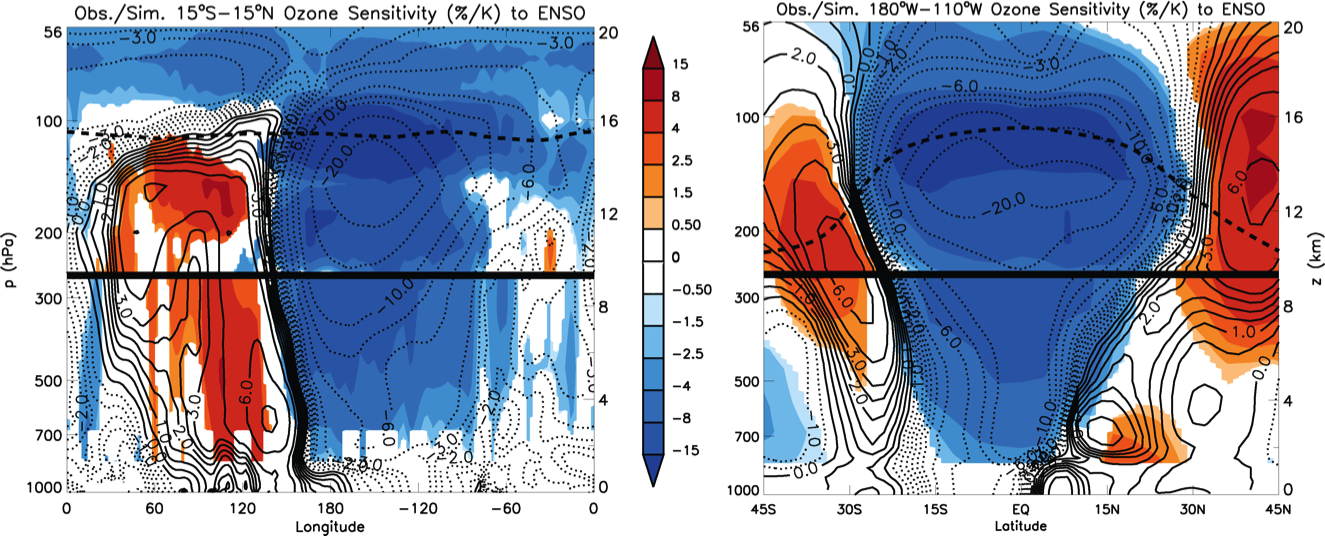
Figure 1. Left: Ozone sensitivity (%/K) to ENSO over the tropics (averaging from 15S-15N) from MLS and TES measurements shown as color filled contours overlaid by GEOS CCM simulated (black contours) ozone sensitivity to ENSO. Right: Ozone sensitivity (%/K) to ENSO over the eastern and central Pacific (averaging from 180W-110W). The dashed black curve is the simulated tropopause.

North Pacific Sea Surface Temperatures Affect the Arctic Winter Climate

Observations suggest that anomalously high sea surface temperatures (SSTs) in the North Pacific may have led to the sustained period of low temperatures and record-breaking ozone depletion that took place in the Arctic stratosphere in spring 2011. However, because the Arctic stratosphere is highly variable, and because the observational record is short, it is not possible to attribute the precise causes of the stratospheric conditions in 2011.

Differences between two sets of model simulations isolate the impact of North Pacific sea surface temperatures (SSTs) on the Arctic winter climate. One set of extended winter season forecasts, or ensemble, is forced by unusually high SSTs in the North Pacific, while in the second ensemble SSTs in the North Pacific are unusually low. Differences between the High and Low ensembles suggest that the lower atmosphere responds to changes in North Pacific SSTs, in particular a weakening of the Aleutian low. The relative change in tropospheric circulation inhibits the propagation of large-scale, or planetary, waves into the stratosphere, in turn reducing polar stratospheric temperatures in mid- and late winter. Also, elevated North Pacific SSTs, associated with relatively colder and more stable Arctic stratospheric winters, greatly reduce the number of mid-winter sudden stratospheric warming events.

Arctic ozone depletion occurs in the presence of polar stratospheric clouds, which form at very low temperatures. Thus, relatively more ozone depletion occurs in winters when the Arctic lower stratosphere is relatively cold, such as when North Pacific SSTs are elevated. In April, polar reduction of ozone shifts to Europe and the Siberian sector, increasing the UV index, while ozone increases in the Canadian sector, decreasing the UV index.

While model simulations support the hypothesis that anomalously warm North Pacific SSTs contributed to the low temperatures and ozone depletion observed in 2011, elevated North Pacific SSTs alone do not predict polar stratospheric conditions in late winter. Random atmospheric variability also plays a role.

Citation:
Hurwitz, M.M., P.A. Newman, and C.I. Garfinkel, 2012. On the Influence of North Pacific Sea Surface Temperatures on the Arctic Winter Climate. J. Geophys. Res., 117, D19110, DOI: 10.1029/2012JD017819.

Arctic Winter Climate Figure 1

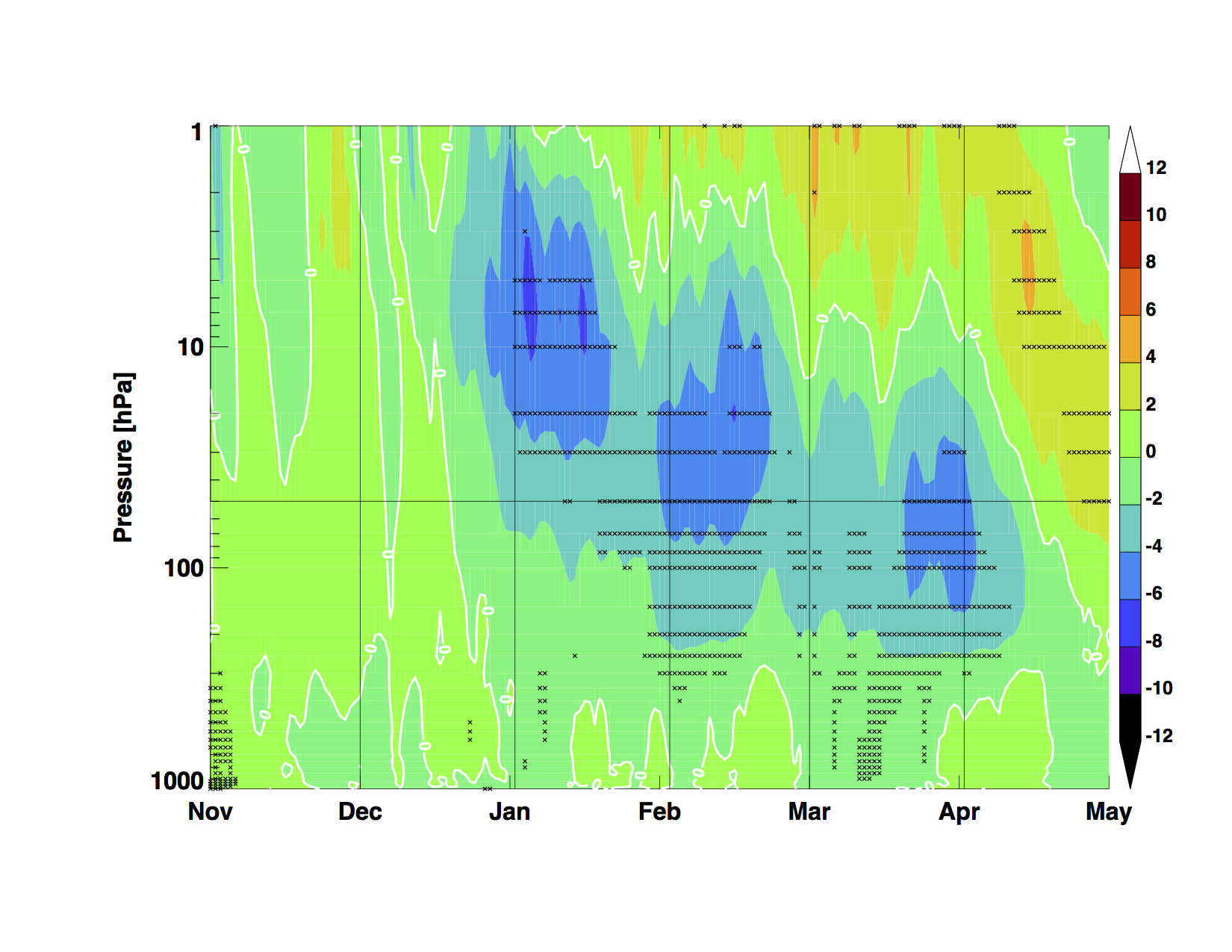
Figure 1. The relative cooling of the Arctic stratosphere due associated with relatively warmer North Pacific SSTs, as modeled in the GEOSCCM (Version 2).

Seasonal Variations of Stratospheric Age Spectra in GEOSCCM

There are many pathways for an air parcel to travel from the troposphere to the stratosphere, each of which takes different time. The distribution of all the possible transient times, i.e. the stratospheric age spectrum, contains important information on transport characteristics. However, it is computationally very expensive to compute seasonally varying age spectra, and previous studies have focused mainly on the annual mean properties of the age spectra. To date our knowledge of the seasonality of the stratospheric age spectra is very limited.

In this study we investigate the seasonal variations of the stratospheric age spectra in the Goddard Earth Observing System Chemistry Climate Model (GEOSCCM). We introduce a method to significantly reduce the computational cost for calculating seasonally dependent age spectra. Our simulations show that stratospheric age spectra in GEOSCCM have strong seasonal cycles and the seasonal cycles change with latitude and height. In the lower stratosphere extratropics, the average transit times and the most probable transit times in the winter/early spring spectra are more than twice as old as those in the summer/early fall spectra. But the seasonal cycle in the subtropical lower stratosphere is nearly out of phase with that in the extratropics. In the middle and upper stratosphere, significant seasonal variations occur in the subtropics. The spectral shapes also show dramatic seasonal change, especially at high latitudes. These seasonal variations reflect the seasonal evolution of the slow Brewer-Dobson circulation (with timescale of years) and the fast isentropic mixing (with timescale of days to months).

Citation:
Li, F., D. W. Waugh, A.R. Douglass, P. A. Newman, S. Pawson, R.S. Stolarski, S.E. Strahan, and J. E. Nielsen, 2012. Seasonal variations of stratospheric age spectra in the Goddard Earth Observing System Chemistry Climate Model (GEOSCCM). J. Geophys. Res, 117, D05134, DOI: 10.1029/2011JD016877.

Age Spectra Variation Figure 1

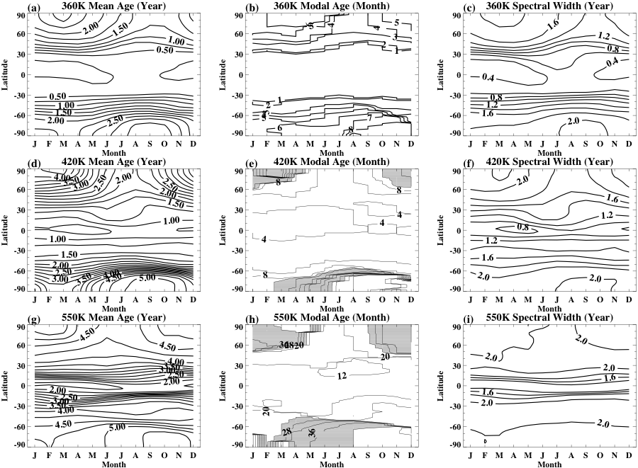
Figure 1. This figure shows the seasonal evolution of the mean age, modal age and spectral width. All three spectral parameters show similar seasonal variations with smaller values in summer/early fall than winter/early spring.

Investigations of Aerosol Impacts on Climate

Atmospheric aerosols are small, airborne particles that reside in the atmosphere for time-periods of up to one week. They are from diverse sources such as from the tail pipe of your car to dust and sea spray whipped up by the wind. Their chemical properties are similarly diverse. Some aerosols grow in humid air or mix with particles of other types, and aerosols are the nuclei of the droplets that make up clouds. Just as aerosols are complex, their interactions with the climate are also complex. Overall, atmospheric aerosols cool the Earth's surface by reflecting sunlight back to space. Some aerosols such as dust and soot, however, also absorb a portion of the sunlight that hits them. As a result, they can heat up the atmosphere, and this heating can decrease the humidity in the air and contribute to the "burn-off" of clouds. Removing these reflective clouds from the climate system actually warms the surface, opposing the overall effect of the aerosols themselves.

The aerosol lifecycle is tightly linked to the climate system, as the climate influences how aerosols are put into and removed from the atmosphere, their transport, and how their physical and chemical properties change. The extremely complex nature of these diverse particles makes modeling their climate interactions difficult. In fact, the International Panel on Climate Change (IPCC) regards aerosols to be one of the largest remaining uncertainties in our understanding of human-induced climate change.

In this study we investigate two different methods for including aerosol-climate interactions in climate models. A fully interactive aerosol module is implemented in the NASA GEOS-5 climate model. In one set of simulations, the aerosols evolve consistently within the model climate. In a second, less computationally intensive, set of simulations we run the climate model but prescribe monthly varying aerosol fields derived from the first set of experiments. By comparing these simulations, we can see the importance of aerosol-meteorology coupling on the simulated climate.

We found that removing the coupling between aerosols and meteorology causes a positive feedback on climate; that is, there is more cooling of the climate in the simulations based on prescribing the monthly varying aerosols. This is because removing coupling artificially removes the correlations that exist between the mass of atmospheric aerosols and humidity, particularly over the ocean. As a result, when the aerosols are prescribed and there is no coupling, variability in humidity causes aerosol particles to grow and become more reflective, which increases the amount of sunlight reflected back to space and cools the climate. This research indicates that aerosol-climate coupling in aerosol modeling can produce significant differences in climate response.

Citation:
Randles C, P. Colarco, A. da Silva, 2013. Direct and semi-direct aerosol effects in the NASA GEOS-5 AGCM: aerosol-climate interactions due to prognostic versus prescribed aerosols. J. Geophys. Res., 118, 149-169, DOI: 10.1029/2012JD018388.

Aerosol Figure 1

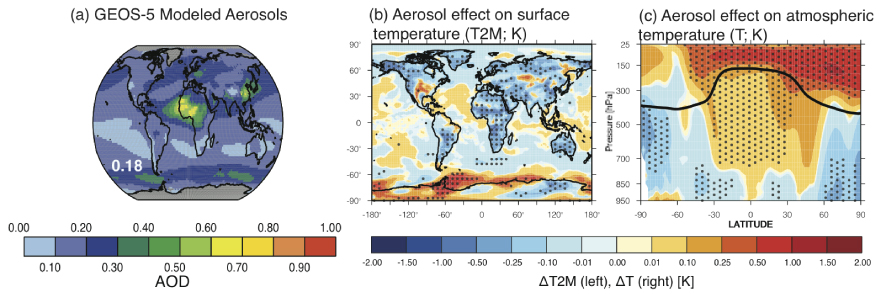
Figure 1. Aerosol-climate simulations in the GEOS-5 CCM. (a) The global distribution of simulated aerosols, where the aerosol optical depth (AOD) is an optical measurement of the amount of aerosol. The highest concentrations of aerosols are over the dusty region of northern Africa and the polluted and dusty regions of south and east Asia. (b) Because they reflect solar radiation back to space, aerosols generally cool the 2-m air temperature over land (the black dots show where these temperature changes are statistically significant). We do not simulate ocean circulation with this model so aerosol impacts on surface air temperature are small over the ocean. (c) Absorbing aerosols such as dust and black carbon contribute to a warming of the tropical atmosphere and lower stratosphere.

Atmospheric Response to the 11-Year Solar Cycle

As the Sun is the ultimate source of virtually all the energy that heats the atmosphere and surface of the Earth, it is not surprising that people for centuries have asked the question "Could changes in the amount of energy coming from the Sun be responsible for changes in the Earth's climate?" Galileo was acutely aware that there were changes in the appearance of the Sun, with his famous observations of sunspots. Sunspot number is one of several proxies of solar activity that have been found to correlate with climate parameters. Although solar forcing of climate is presently thought to be an order of magnitude smaller than anthropogenic factors, our scientific understanding of the solar influence is low. To fully understand the Sun-climate connection, we must understand both the variability of the Sun and how the Earth system responds to such variations.

NASA has been directly observing the solar output from space since the 1970s. The Sun is thus known to vary on a range of timescales, from days to years and even longer. One of the most salient variations is the 11-year solar cycle. Although the total solar irradiance (TSI) varies by less than 0.1% over the course of a solar cycle, the variation at particular wavelengths can be much larger, for example at ultraviolet (UV) wavelengths, having important implications for stratospheric chemistry and circulation that are in turn coupled to climate close to the surface. NASA's SOlar Radiation & Climate Experiment (SORCE) mission has been making critical measurements of solar spectral irradiance (SSI), or solar energy as a function of wavelength, since 2004, spanning parts of solar cycles 23 and 24. A key and controversial SORCE finding is the suggestion that the UV solar cycle variations are several times larger than previously accepted based on past measurements. Several studies have been published recently in the US and Europe that combine the SORCE SSI with atmospheric models to predict potential climate impacts of this larger UV variability. These studies suggest that, if the SORCE SSI is correct, the atmospheric response to the solar cycle could be very different than we expected.

In our new paper, we study the mechanisms of atmospheric response to the solar cycle as simulated in two state-of-the-art chemistry-climate models (CCMs): the 3-D Goddard Earth Observing System (GEOS) CCM and the Goddard Space Flight Center (GSFC) 2-D coupled model. We compare and contrast how the model atmosphere responds to both the long-accepted SSI typically used in climate projections, developed at the Naval Research Laboratory, and the new SORCE SSI. The solar cycle in SSI is a very challenging measurement, and the purpose of this paper is not to substantiate or disprove the SORCE measurements but rather to contribute to a better, more generalized understanding of solar effects.

Our study explains why GCMs without coupled chemistry underestimate the temperature response to the solar cycle. Further, we show how different wavelength regions of the solar spectrum contribute to the middle atmosphere ozone response (see Fig. 2), and how the solar cycle signals derived from the SORCE instruments measuring these different regions lead to surprising model outcomes (see Fig. 1).

Although the solar forcing of climate is presently thought to be an order of magnitude smaller than anthropogenic factors, our scientific understanding of the solar influence is low. This study provides a path forward for a more general understanding and prediction of the atmosphere/climate response to solar variations.

Citation:
Swartz, W. H., R. S. Stolarski, L. D. Oman, E. L. Fleming and C. H. Jackman, 2012. Middle atmosphere response to different descriptions of the 11-yr solar cycle in spectral irradiance in a chemistry-climate model. Atmos. Chem. Phys., 12, 5937-5948, DOI: 10.5194/acp-12-5937-2012.

Solar Cycle Figure 1

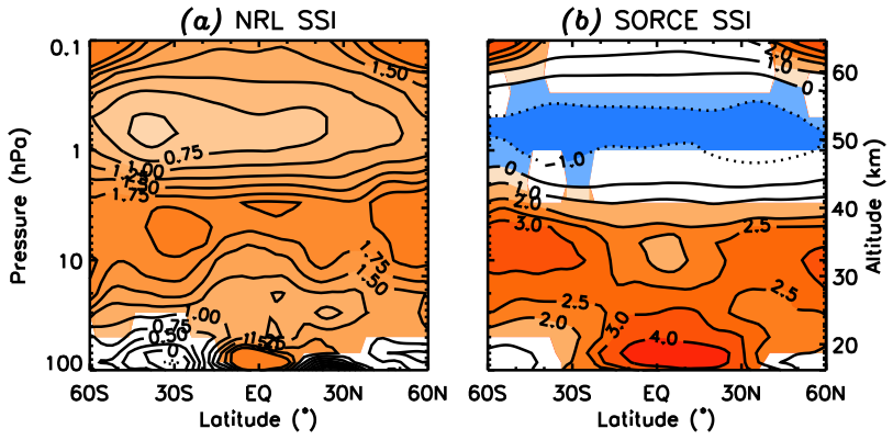
Figure 1. Simulated response of ozone to the solar cycle (O3 change (%) for solar maximum vs. minimum conditions) in the GEOSCCM using the (a) NRL and (b) SORCE solar flux. The colored (non-white) portions of the plots indicate regions where the ozone response is statistically significant. At the top of the stratosphere near 50 km, the SORCE solar flux produces net ozone loss in the model (blue shaded region), which is unexpected.

Solar Cycle Figure 2

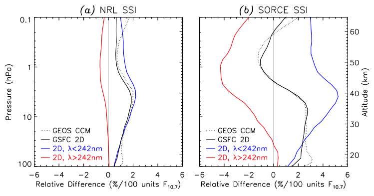
Figure 2. Simulated response of ozone to the solar cycle in the GSFC 2-D model in different wavelength ranges. The model shows how the solar cycle at wavelengths shorter than 242 nm lead to net production of ozone (in blue), while longer wavelengths lead to ozone loss (in red).

Impacts of El Niño Events on the Antarctic Stratosphere

Conventional El Niño events are characterized by warmer than average sea surface temperatures in the equatorial eastern Pacific Ocean and by an eastward shift in atmospheric convection from Asia toward the central Pacific. The largest El Niño event in recent decades occurred in 1997/1998. The El Niño signal propagates polewards and upwards as large-scale atmospheric waves, leading to unusual weather worldwide and changing conditions in the stratosphere. While the Arctic stratosphere warms in response to these conventional or “cold tongue” type of El Niño events, the Antarctic stratosphere is unaffected.

Recently, a second type of El Niño event has been identified. During “warm pool” El Niño events, sea surface temperatures in the central Pacific are warmer than average. This study identifies a robust warming of the Antarctic stratosphere in Southern Hemisphere spring and summer, in response to “warm pool” El Niño events, using atmospheric data from 1979 to 2009. The Antarctic warming associated with “warm pool” El Niño events is most pronounced when these events are coincident with westward winds in the tropical lower and middle stratosphere. Westward winds may enhance wave activity in the subtropical troposphere and/or push wave energy toward polar latitudes. Because of the small number of observed El Niño events, model experiments will be required to better understand how tropical winds affect the Antarctic response to “warm pool” El Niño events.

Citation:
Hurwitz, M. M., P. A. Newman, L. D. Oman, and A. M. Molod, 2011. Response of the Antarctic Stratosphere to Two Types of El Niño Events. J. Atmos. Sci., 68, DOI: 10.1175/2011JAS3606.1.

El Nino Figure 1

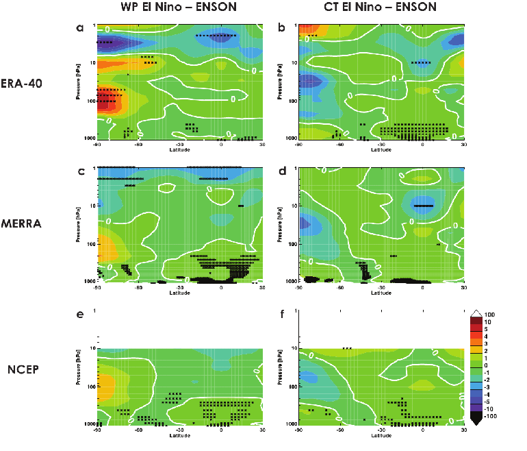
Figure 1. Latitude-height cross-sections of November/December mean temperature differences (K), from a composite of ENSO neutral events, in WP El Niño events (a, c, e) and CT El Niño events (b, d, f). White contours indicate zero difference from the composite of ENSO neutral events. Black Xs indicate differences that are significant at the 95% confidence level.

Unusual Dynamical Conditions in the Arctic Stratosphere in March 2011

In March 2011, the Arctic stratosphere was much colder than usual, leading to severe polar ozone depletion.

March temperature in the Arctic stratosphere is highly correlated with tropospheric wave forcing in February (Newman et al., 2001). Meteorological reanalyses show that wave forcing in 2011 was much weaker than usual, consistent with the unusually cold conditions. Similarly weak wave forcing and March temperatures were observed in 1997.

Dynamical conditions that are known to reduce wave activity and cool the Arctic stratosphere in mid-winter (specifically, La Nina and QBO-westerly; see Garfinkel et al., 2010) persisted throughout the 2010-2011 winter season. However, they do not explain the unusually cold Arctic stratosphere in March 2011.

Sea surface temperatures (SSTs) in the North Pacific were warmer than usual in the late winter in both 1997 and 2011. The positive phase of this "subarctic SST mode" is associated with a cooler Arctic stratosphere in March. This result provides new evidence for interactions between the ocean and stratosphere and motivates a modeling study of the role of extra-tropical SSTs on Arctic variability.

Citation 1:
Hurwitz, M., P. A. Newman, and C. I. Garfinkel, 2011. The Arctic vortex in March 2011: a dynamical perspective. Atmos. Chem. Phys., 11, 11447-11453, DOI: 10.5194/acp-11-11447-2011.

Citation 2:
Garfinkel, C. I., D. L. Hartmann, and F. Sassi, 2010. Tropospheric Precursors of Anomalous Northern Hemisphere Stratospheric Polar Vortices. Journal of Climate, 23, 3282-3299, DOI: doi: http://dx.doi.org/10.1175/2010JCLI3010.1

Citation 3:
Newman, P. A., E. R. Nash, and J. E. Rosenfield, 2001. What controls the temperature of the Arctic stratosphere during the spring? Journal of Geophysical Research, 106, 19,999-20,010, DOI: 10.1029/2000JD000061.

august2011

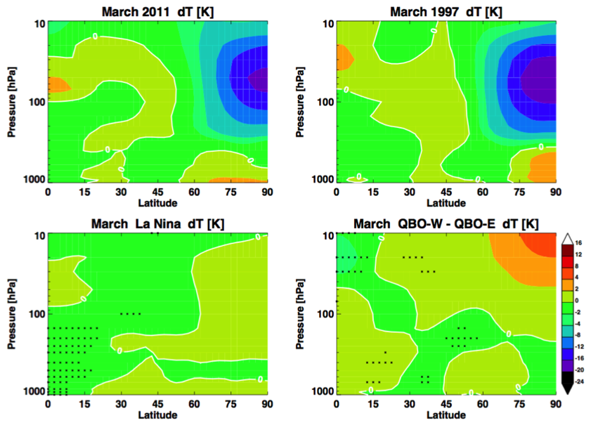
Figure 1. The top two panels show March temperature differences from climatology in the Northern Hemisphere troposphere and stratosphere. In 2011 and 1997, the Arctic stratosphere was approximately 10K colder than usual. The center panels show that typical La Nina and QBO-westerly conditions are not consistent with the cold conditions in March 2011. The lower panel shows that the positive phase of the subarctic SST mode may explain the unusually cold Arctic stratosphere in March 2011.

Ozone and Reactive Nitrogen in Arctic Free Troposhere Determined Primarily by Stratospheric Influx

Ozone in the Arctic troposphere is important as a surface pollutant affecting air quality and a greenhouse gas that contributes to Arctic warming.

Currently there lacks a clear understanding of how each source, e.g. anthropogenic and biomass burning emissions and stratospheric intrusion, contribute to the ozone abundance in the Arctic troposphere.

We analyze the aircraft observations obtained during the NASA ARCTAS aircraft mission to examine ozone and reactive nitrogen. The latter determines the production efficiency of ozone in the troposphere, in the Arctic and sub-Arctic region and their source attribution. We find:
i) While anthropogenic, biomass burning, and convective air masses contain elevated NOx and hydrocarbons (precursors of O3), and display high O3 production rates, they do not contribute significantly to O3 in the Arctic troposphere.
ii) Stratospheric air, when injected into the troposphere, is a major source of O3, NOx, as well as NOx reservoir species (HNO3, PAN) in the Arctic upper troposphere. The STE air masses is also the main driver of net ozone formation in the Arctic upper troposphere.

Citation:
Liang, Q., J. M. Rodriguez, A. R. Douglass, J. H. Crawford, E. Apel, H. Bian, D. R. Blake, W. Brune, M. Chin, P. R. Colarco, A. da Silva, G. S. Diskin, B. N. Duncan, L. G. Huey, D. J. Knapp, D. D. Montzka, J. E. Nielsen, J. R. Olson, S. Pawson, A. J. Weinheimer, 2011. Reactive Nitrogen, Ozone and Ozone production in the Arctic Troposphere and the Impact of Stratosphere-Troposphere Exchange. Atmos. Chem. Phys., 11, 13181-13199, DOI: 10.5194/acp-11-13181-2011 .

ARCTAS_1

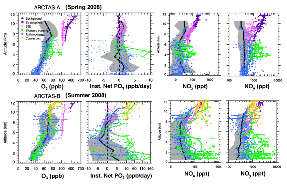
Figure 1. Upper panels: Vertical profiles of O3, instantaneous net O3 production rates , NOx, and NOy (=NOx+PAN+HNO3) during ARCTAS-A, Spring 2008. Black lines show the mean 1-km binned values in background air masses sampled by the NASA DC-8 aircraft during ARCTAS-A. We highlight the individual air masses using color symbols: stratosphere (purple), Stratosphere-Troposphere Exchange (STE) (lilac), anthropogenic pollution (blue), biomass burning (green), and convection/lightning (yellow). The solid color lines indicate the vertical mean profiles of individual air masses. The lower panels are the same as the upper panels but for ARCTAS-B, Summer 2008, instead.

The Response of Tropical Tropospheric Ozone to El Niño Southern Oscillation (ENSO)

El Niño Southern Oscillation (ENSO) is the dominant mode of tropical variability on interannual timescales. It is well known to have a significant influence on the atmospheric circulation of the tropical Pacific. Its influence however, extends beyond the thermal and dynamical and into the chemical composition of the troposphere, the lowest layer of the atmosphere. One key atmospheric gas that past studies have shown to be influenced by ENSO is ozone. It is important to determine how and why ozone varies in the troposphere because of its significant influence on the atmospheres radiative heating budget.

A new study by scientists at NASA's Goddard Space Flight Center (GSFC) and Johns Hopkins University used a comprehensive chemistry-climate model to show the impact that ENSO has on tropical tropospheric ozone. Our simulation has successfully reproduced the Ozone ENSO Index (OEI), which results from ozone changes over the Pacific Ocean. This OEI also provides an excellent measure of chemistry-climate models response to ENSO variability and can be used in their evaluation. Our study further examines the 3-dimensional structure of ENSO related ozone variations and compares this to those obtained from the Southern Hemisphere Additional Ozonesondes (SHADOZ) measurements.

The technique used in this study helps to view tropospheric ozone variability in a climate context rather than as individual case studies. Using a combination of simulation and atmospheric measurements the far-reaching affects of ENSO continue to be unraveled. This work is part of a larger chemistry climate project at GSFC with the ultimate goal of using observations and computer simulations to improve our knowledge of Earth's climate system.

Citation:
Oman, L.D., J.R. Ziemke, A.R. Douglass, D. W. Waugh, C. Lang, J.M. Rodriguez, and J. E. Nielsen, 2011. The response of tropical tropospheric ozone to ENSO. Geophys. Res. Lett, 38(L13706), DOI: 10.1029/GL047865.

OEI Time Series Figure 1

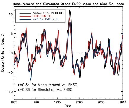
Figure 1. The Ozone ENSO Index (OEI) is derived by averaging monthly tropospheric column ozone over two broad regions of the western and eastern Pacific (15S-15N, 70E-140E, and 15S-15N, 110W-180W, respectively) and taking their difference (western minus eastern Pacific). The time series is then deseasonalized and smoothed with a 3-month running average (black curve). We used the Goddard Earth Observing System (GEOS) version 5 coupled to the comprehensive Global Modeling Initiative (GMI) stratosphere-troposphere chemical mechanism to simulate the impact of observed sea surface temperature changes on tropospheric ozone concentrations. This simulation used fixed in time natural and anthropogenic emission sources to evaluate the variability due to sea surface temperature changes. Using the tropospheric column ozone amounts from the simulation averaged over the same two regions the values were differenced, deseasonalized, and smoothed using a 3-month running average (red curve). Niño 3.4 Index is shown as the blue curve multiplied by 3 for scaling. All three times series are strongly correlated over the 25 year period with Measurement vs. ENSO correlation of 0.84 and Simulation vs. ENSO correlation of 0.86.

Breakup of the Antarctic Polar Vortex

In mid-winter, winds circle the globe at speeds greater than 200 km/hr (~130mph) in the middle atmosphere. This strong jet bounds the region known as the polar vortex. The presence of the Antarctic polar vortex is a key ingredient in the formation of the ozone hole, because the air inside the vortex is cold and isolated from lower latitudes, creating ideal conditions for large-scale chemical ozone depletion.

Many atmospheric models are not able to reproduce observed winds in the middle atmosphere. Specifically, the polar vortices tend to break down too late and peak wind speeds are higher than observed. This study finds that the delayed break-up of the Antarctic polar vortex is due to weaker-than-observed wave driving from the lower atmosphere during the October-November period. The delayed break-up of the Antarctic polar vortex changes the temperature structure of the middle atmosphere, which biases the amount of chemical ozone depletion that can occur in late winter and spring. Also, the extended lifetime of the polar vortex strengthens the overturning circulation cell in the middle atmosphere, changing the amount of ozone, methane and other chemical species that is transported from low to high latitudes.

Understanding model weaknesses and improving the modeled polar vortices will be necessary for accurate predictions of ozone recovery in the coming century.

Citation:
Hurwitz, M. M., P. A. Newman, F. Li, L. D. Oman, O. Morgenstern, P. Braesicke, and J. A. Pyle, 2010. Assessment of the breakup of the Antarctic polar vortex in two new chemistry-climate models. J. Geophys. Res., 115, D07105, DOI: 10.1029/2009JD012788.

Break Up Figure 1

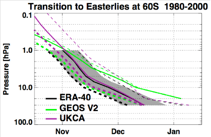
Figure 1. Timing of the transition to easterlies (i.e., vortex breakup) at 60S during the 1980\u20132000 period, as a function of altitude. The black line shows the mean date of the transition from westerlies to easterlies for the ERA-40 reanalysis data set; the gray shading indicates the range of variability between 1980 and 2000. The solid lines (green, GEOS V2; purple, UKCA) show the simulated mean date of the transition to easterlies between 1980 and 2000. The thick (thin) dashed lines show the mean date of the transition to easterlies in cases when the 100 hPa heat flux between 40°S and 80°S is high (low).

Future Temperature Trends in the Antarctic Stratosphere

This study examines trends in Antarctic temperature and APSC, a temperature proxy for the area of polar stratospheric clouds, in an ensemble of Goddard Earth Observing System (GEOS) chemistry-climate model (CCM) simulations of the 21st century. A selection of greenhouse gas, ozone-depleting substance, and sea surface temperature scenarios is used to test the trend sensitivity to these parameters. One scenario is used to compare temperature trends in two versions of the GEOSCCM. An extended austral winter season is examined in detail. In May, June and July, the expected future increase in CO2-related radiative cooling drives temperature trends in the Antarctic lower stratosphere. At 50 hPa, a 1-3 K cooling is expected between 2000 and 2100. Ozone levels increase, despite this robust cooling signal and the consequent increase in APSC, suggesting the enhancement of stratospheric transport in future. In the lower stratosphere, the choice of climate change scenarios does not affect the magnitude of the early winter cooling. Mid-winter temperature trends are generally small. In October, APSC trends have the same sign as the prescribed halogen trends. That is, there are negative APSC trends in “realistic future ” simulations, where halogen loading decreases in accordance with the Montreal Protocol and CO2 continues to increase. In these simulations, the speed of ozone recovery is not influenced by either the choice of sea surface temperature and greenhouse gas scenarios, or by the model version.

Citation:
Hurwitz, M. M. and P. A. Newman (2010). 21st century trends in Antarctic temperature and polar stratospheric cloud (PSC) area in the GEOS chemistry-climate model. J. Geophys. Res., 115, D19109, DOI: 10.1029/2009JD013397.

Temp Trends Figure 1

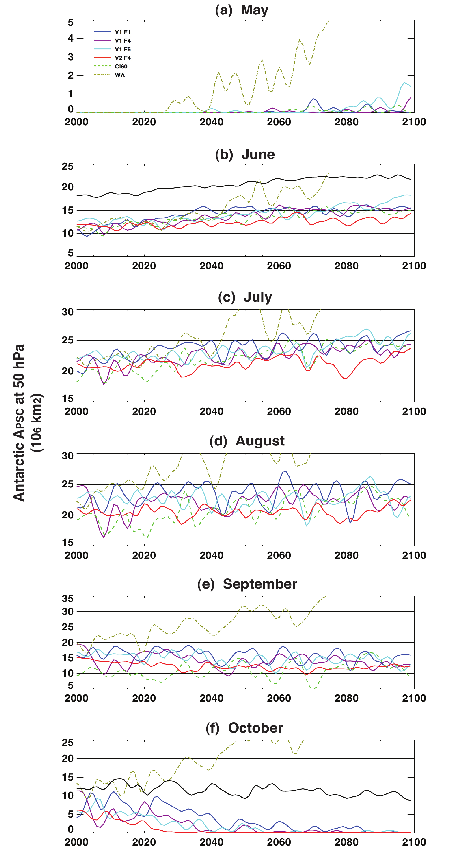
Figure 1. APSC at 50 hPa (106 km2) between and 2000 and 2099. Shown are GEOSCCM simulations V1 F1 (blue), V1 F4 (purple), V1 F5 (cyan), V2 F4 (red), Cl60 (green) and WA (brown). CMAM ensemble mean timeseries in mid\u2013June (b) and mid\u2013October (f) are shown in black. Solid lines denote "realistic future" simulations. Note the different vertical scales in each of the panels. Three iterations of a 1-2-1 smoothing algorithm have been applied to all timeseries.

Narrowing of the Tropical Upwelling in the Stratosphere and Troposphere in Chemistry-Climate Model Simulations of the 21st Century

Strong evidence of a tropical belt expansion during the last three decades has been reported recently. Observational studies have shown that the Tropics have widened by more than two degrees latitude since 1979. Expansion of the Tropics in the 20th and 21st Century is also simulated by the Intergovernmental Panel on Climate Change (IPCC) Fourth Assessment Report (AR4) models. The widening of the Tropics is closely linked to the expansion of the Hadley cell's sinking branches. Because the Hadley cell's sinking branches cause the subtropical deserts, a widening of the Hadley cell means that the subtropical dry zones are moving toward more populated areas, including the American southwest, southern Australia and the Mediterranean basin. In addition, the tropical belt expansion is associated with changes in jet streams and storm tracks, and therefore has important implications in climate change. Understanding the mechanisms responsible for the tropical belt widening, particularly for the expansion of the Hadley cell, is an active research area.

This work investigates two important aspects of tropical expansion that have not been examined in previous studies. The first is the width of the stratospheric circulation (the Brewer-Dobson circulation) under global warming: it is important to understand whether tropical expansion extends into the stratosphere. The second topic is the width of the ascending branch of the Hadley cell: studying changes in the Hadley cell's upwelling will help to understand what causes the expansion of the Hadley cell's sink branch. These two topics were investigated using simulations of the 21st century from the Goddard Earth Observing System Coupled Chemistry Climate Model (GEOSCCM). The model results project a narrowing of the tropical upwelling region in the troposphere and lower stratosphere. However, the mechanisms for the narrowing of the upwelling branch of the Brewer-Dobson and the Hadley circulation are different. The narrowing of the upwelling of the Brewer-Dobson circulation in the lower stratosphere is due to the strengthening and equatorward shift of the subtropical jets, which enhances equatorward propagation of midlatitude eddies. On the other hand, the narrowing of the Hadley cell's ascending branch is caused by suppressed equatorward propagation of eddies, possibly a result of enhanced static stability in the troposphere. The reduced eddy wave activity causes anomalous eastward wave forcing in the subtropical upper troposphere, which drives an indirect circulation whose sinking branch narrows the tropical upwelling region.

Citation:
Li, F., R.S. Stolarski, S. Pawson, P. A. Newman, and D. Waugh, 2010. Narrowing of the upwelling branch of the Brewer-Dobson circulation and Hadley cell in chemistry-climate model simulations of the 21st century. Geophys. Res. Lett, 37(L13702), DOI: 10.1029/2010GL043718.

Tropical Narrowing Figure 1

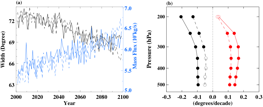
Figure 1. The right panel shows that while the strength of the tropical upwelling in the lower stratosphere (blue lines) increases, the width of the upwelling area decreases (black lines) in the GEOSCCM 21st simulations. The left panel shows that the outer boundary of the Hadley cell (red lines) expands poleward, but the width of the rising branch of the Hadley cell (black line) decreases.

Ozone Hole and Southern Hemisphere Circulation Change

The Antarctic ozone hole impacts both tropospheric and stratospheric climate, particularly in summer season. We investigated climate change in 1960-2060 using a chemistry-climate model. The scientific questions we try to address are: What is role of the ozone hole in climate change? Are circulation changes in the troposphere and stratosphere related to each other?

The ozone hole significantly changes the stratospheric circulation: it strengthens the Antarctic mass downwelling by more than 1/3 and it increases the polar jet by 50% in summer. The ozone hole also strongly impacts the tropospheric circulation pattern, causing a poleward movement of the tropical jet and strengthening the jet by 25%. Circulation changes in the troposphere and stratosphere are strongly correlated.

This study has identified ozone hole's role in driving circulation changes in the stratosphere and troposphere. These results imply that the projected ozone recovery in the latter half of this century will strongly impact future climate change. On the other hand, an enhanced stratospheric circulation will significantly affect ozone distribution in the post-CFC era. Furthermore, an accelerated stratospheric transport circulation will increase stratosphere-troposphere exchange, which would affect tropospheric air quality, for example, by bringing more stratospheric ozone into the troposphere. Thus, our research will help to understand ozone recovery and air pollution in a changing climate.

Citation:
Li, F., P.A. Newman, and R.S. Stolarski, 2010. Relationships between the Brewer-Dobson circulation and the southern annular mode during austral summer in coupled chemistry-climate model simulations. J. Geophys. Res., 115(D15106), DOI: 10.1029/2009JD012876.

Ozone Circulation Change
Figure 1

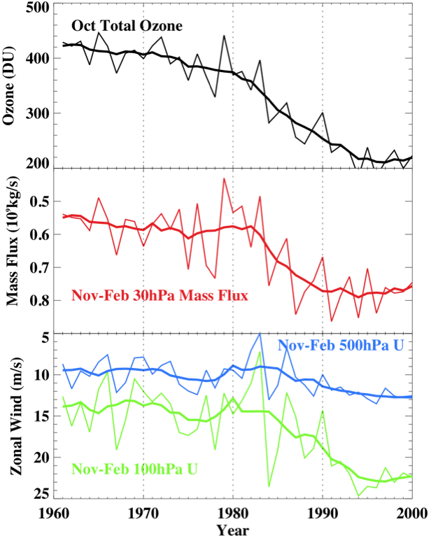
Figure 1. Time series of (top) October Antarctic total ozone, (middle) Nov-Feb mean Southern Hemisphere stratospheric mass flux, and (bottom) the Nov-Feb mean subpolar zonal wind at 5 km (blue) and 16 km (green). Thick curves are 7-year running average mean. The top and middle panels show high correlation between the ozone hole and the acceleration of the stratospheric mean transport circulation. The lower panel indicates that ozone hole impacts the subpolar jets in the troposphere and stratosphere. Changes in the circumpolar jets are a measure of the Southern Annular mode, a dominant circulation pattern in the troposphere. In contrast, in an experiment that does not include ozone depletion, neither the stratospheric circulation nor the Southern Annular Mode has significant trends (not shown). These model results indicate that Antarctic ozone depletion is a major driver for both the stratospheric and tropospheric climate change in the Southern Hemisphere in the last 3 decades.

Investigations of 21st Century Ozone

Future ozone evolution and the factors that dominate that evolution is a primary topic in current atmospheric chemistry research. Ozone is a very important atmospheric gas that absorbs damaging ultraviolet radiation, so changes in the total amount above us can have important consequences for our biosphere. The ability of ozone to absorb sunlight, mainly in the ultraviolet but also in the visible range, as well as some of Earth's outgoing longwave radiation causes heating of the upper layers of our atmosphere which can have many impacts, including changes in wind patterns.

A new study by scientists at NASA's Goddard Space Flight Center (GSFC) and Johns Hopkins University used a state-of-the-art chemistry climate model to explain what could potentially be driving changes in ozone in the upper levels of our atmosphere over the 21st century. They found that in the upper stratosphere, the region from 20 to 30 miles above the surface, the reduction in chlorine and cooling temperatures contribute about equally to future increases in ozone in the tropics. The future reduction in chlorine, which is formed mostly from the breakdown of chlorofluorocarbons (CFC's), is the expected result of the successful implementation of the Montreal Protocol and its subsequent amendments and adjustments. The continued cooling of the stratosphere is a response largely caused by increasing concentrations of carbon dioxide (CO2), which is opposite of the warming that CO2 causes closer to the surface.

The technique that was developed in this study helps to separate the relative contributions of several factors that can influence ozone and can be applied to a wide range of greenhouse gas scenarios as well as to other chemistry climate models. This method can potentially be very useful in explaining differences in ozone trends among models and will be used in an upcoming assessment for this purpose. This work is part of a larger chemistry climate project at GSFC with the ultimate goal of using observations and computer modeling to improve our knowledge of Earth's climate system.

Citation:
Oman, L. D., D. W. Waugh, S. R. Kawa, R. S. Stolarski, A. R. Douglass, and P. A. Newman, 2010. Mechanisms and feedbacks causing changes in upper stratospheric ozone in the 21st century. J. Geophys. Res., 115, D05303, DOI: 10.1029/D012397.

o3_21cent Figure 1

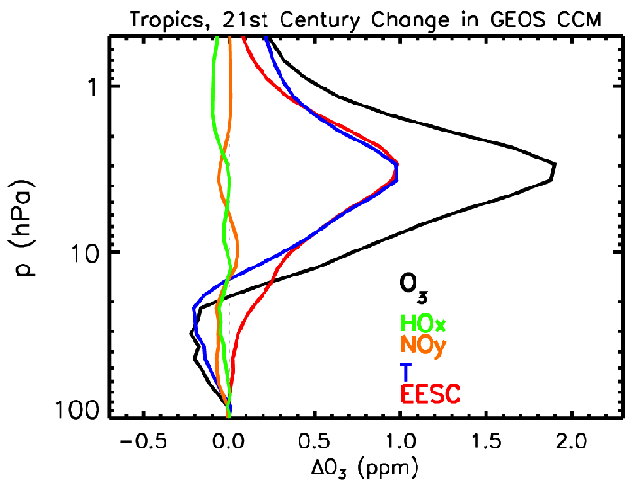
Figure 1. This figure shows the vertical variation of trends in ozone (solid black curve) and individual contribution of different mechanisms over the tropics (10°S-10°N) for the 21st century in GEOSCCM. The dominate impacts are from temperature (T, blue curve) changes and chlorine and bromine (EESC, red curve) changes with negligible contribution from hydrogen (HOx, green curve) and nitrogen (NOy, orange curve) oxides for the A1b (mid-range) greenhouse gas scenario.

Separation of Chemistry and Climate Signals

Abstract
The temperature of the stratosphere has decreased over the past several decades. Two causes contribute to that decrease: well-mixed greenhouse gases (GHGs) and ozone-depleting substances (ODSs). This paper addresses the attribution of temperature decreases to these two causes and the implications of that attribution for the future evolution of stratospheric temperature. Time series analysis is applied to simulations of the Goddard Earth Observing System Chemistry-Climate Model (GEOSCCM) to separate the contributions of GHGs from those of ODSs based on their different time-dependent signatures. The analysis indicates that about 60%-70% of the temperature decrease of the past two decades in the upper stratosphere near 1 hPa and in the lower midlatitude stratosphere near 50 hPa resulted from changes attributable to ODSs, primarily through their impact on ozone. As ozone recovers over the next several decades, the temperature should continue to decrease in the middle and upper stratosphere because of GHG increases. The time series of observed temperature in the upper stratosphere is approaching the length needed to separate the effects of ozone-depleting substances from those of greenhouse gases using temperature time series data.

Citation:
Stolarski, R.S., A.R. Douglass, P.A. Newman, S. Pawson, and M.R. Schoeberl, 2010. Relative Contribution of Greenhouse Gases and Ozone-Depleting Substances to Temperature Trends in the Stratosphere: A Chemistry-Climate Model Study. J. Climate, 23, 28-42, DOI: 10.1175/2009JCLI2955.1.

trend Figure 1

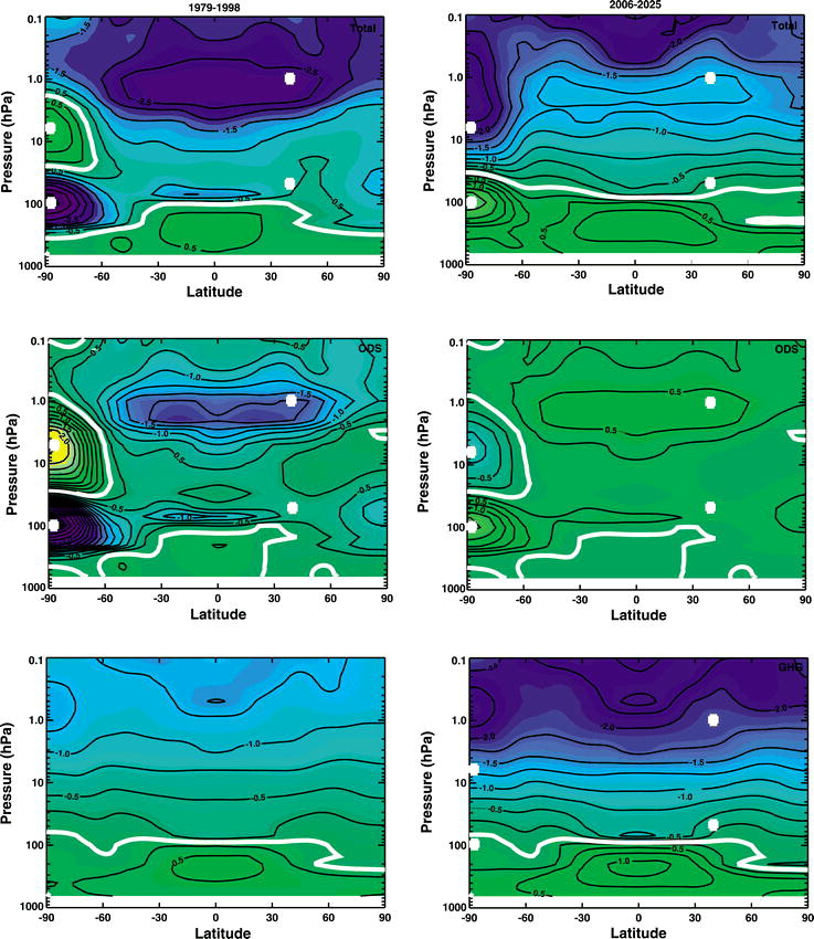
Figure 1. left) Temperature change (K) from 1979 to 1998 and (right) from 2006 to 2025 for GEOSCCM simulations: (top) total temperature change, (middle) change due to ozone-depleting substances, and (bottom) change due to greenhouse gases. Dividing by 2 will give the temperature trends in K decade?1 for each of the 20-yr time periods.

Stratospheric Ozone in the post-CFC Era

The stratospheric ozone layer protects life on the Earth from the Sun's harmful ultraviolet radiation. In the middle 1970s scientists found that this natural shield could be depleted by human made chlorine and bromine containing chemicals, in particular, chlorofluorocarbons (CFCs), which were widely used as refrigerants, foaming agents, and in many other applications. Stratospheric ozone depletion can greatly increase the rates of skin cancer and cataracts, and can significantly diminish global crop yields. By the mid-1980s, clear evidence of ozone depletion was found over Antarctica, the so-called, "Antarctic ozone hole." In response to this threat, governments around the world signed an international agreement, the 1987 Montreal Protocol with its subsequent amendments and adjustments, to phase out CFCs and other ozone-depleting substances (ODS). With the compliance with these agreements, it is projected that the ODS amounts in the stratosphere will return to pre-1980 levels in the 2060s. The ODS level, however, is not the only factor affecting ozone recovery. Changes in temperature and transport in the stratosphere, because of greenhouse gases (GHG), could also have significant impacts on ozone recovery. In this study, using simulations from the Goddard Earth Observing System Coupled Chemistry-Climate Model (GEOSCCM), we try to answer an outstanding scientific question: how does climate change affect ozone recovery?

The model simulations show that the ODS will recover to 1980 values in the 2060s, but stratospheric ozone in the 2060s differs significantly from that in 1980. In fact, the global total ozone levels in 2060 will be higher than in the 1980s with peak increases of 23 DU (6%) in the extratropics, "a super recovery". On the other hand, the tropical column ozone, however, does not recover to 1980 levels up to the end of the simulation in 2100. We found that these post-CFC ozone changes can be largely attributed to climate change. Two mechanisms through which climate change affects ozone recovery have been identified. The first is a "cooling" mechanism that dominates ozone changes in the upper stratosphere (above 30 km). In the upper stratosphere, GHG increases induce a cooling that leads to more ozone because the photochemical reactions that destroy ozone are strongly dependent on temperature. The strong cooling in the upper stratosphere (about 1K/decade) slows the ozone loss reactions by 10-20% in the 2060s and results in an increase in the upper stratospheric ozone of 6 DU. However, this "cooling" mechanism is not important in the lower stratosphere (where most of the ozone resides). The lower stratospheric ozone changes are due to a strengthening of the mean transport circulation, a dynamical response to GHG increase. The stratospheric mean transport circulation redistributes ozone from its source region in the tropics to extratropics. Therefore an enhanced transport decreases tropical ozone but increases extratropical ozone. The total ozone changes are thus determined by the combined effects of these two mechanisms. In the tropics, lower stratospheric ozone decrease due to enhanced transport outweighs upper stratospheric ozone increase, and the tropical total column ozone will not recover to pre-CFC levels. In the extratropics, enhanced transport acts together with upper stratospheric ozone increase to cause a "super recovery".

Citation:
Li, F., R. S. Stolarski, and P. A. Newman, 2009. Stratospheric ozone in the post-CFC era. Atmos. Chem. Phys., 9, 2207-2213, DOI: 10.5194/acp-9-2207-2009.

Post CFCs Figure 1

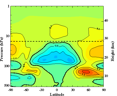
Figure 1. This plot of ozone concentration by latitude and altitude shows the net gain (oranges and reds) and net loss of ozone from years 1975-84 to 2060-69.

Post CFCs Figure 2

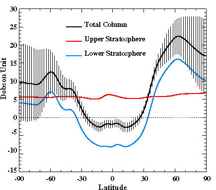
Figure 2. Plot of the change in ozone concentrations by latitude from years 1975-84 to 2060-69 shows a surplus over the high latitudes and a loss near the tropics and equator.

The "World-Avoided" Experiment

Abstract
Ozone depletion by chlorofluorocarbons (CFCs) was first proposed by Molina and Rowland in their 1974 Nature paper. Since that time, the scientific connection between ozone losses and CFCs and other ozone depleting substances (ODSs) has been firmly established with laboratory measurements, atmospheric observations, and modeling studies. This science research led to the implementation of international agreements that largely stopped the production of ODSs. In this study we use a fully-coupled radiation-chemical-dynamical model to simulate a future world where ODSs were never regulated and ODS production grew at an annual rate of 3%. In this "world avoided" simulation, 17% of the globally-averaged column ozone is destroyed by 2020, and 67% is destroyed by 2065 in comparison to 1980. Large ozone depletions in the polar region become year-round rather than just seasonal as is currently observed in the Antarctic ozone hole. Very large temperature decreases are observed in response to circulation changes and decreased shortwave radiation absorption by ozone. Ozone levels in the tropical lower stratosphere remain constant until about 2053 and then collapse to near zero by 2058 as a result of heterogeneous chemical processes (as currently observed in the Antarctic ozone hole). The tropical cooling that triggers the ozone collapse is caused by an increase of the tropical upwelling. In response to ozone changes, ultraviolet radiation increases, more than doubling the erythemal radiation in the northern summer midlatitudes by 2060.

Citation:
Newman P.A., L.D. Oman, A.R. Douglass, E.L. Fleming, S.M. Frith, M.M. Hurwitz, S.R. Kawa, C.H. Jackman, N.A. Krotkov, E.R. Nash, J.E. Nielsen, S. Pawson, R.S. Stolarski, and G.J.M. Velders, 2009. What would have happened to the ozone layer if chlorofluorocarbons (CFCs) had not been regulated? Atmos. Chem. and Phys., 9, 2113-2128, DOI: 10.5194/acp-9-2113-2009.

world_avoided Figure 1

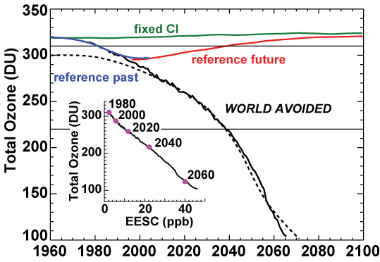
Figure 1. Annual average concentrations of global ozone are shown for the "World Avoided" (solid black), a modeled future with ozone regulation (red), atmospheric chlorine at a fixed amount (green), and a simulation of past observations (blue). The inset shows how ozone concentrations decrease as the amount of chlorine in the atmosphere -- effective equivalent stratospheric chlorine (EESC) -- grows over time.

Long-term Changes in Stratospheric Circulation

The circulation of the stratosphere, the region from 8-30 miles above the surface, is an important part of Earth's climate system. The motions of this region play an integral part in determining the distributions of many trace species, including ozone. Changes in this circulation could potentially act to significantly affect the distribution of ozone as well as substances like chlorine and bromine-containing compounds that destroy ozone, which can impact the timing of the recovery of the ozone layer. To date nearly all climate models predict that the circulation of the stratosphere will become faster over time, but observations have yet to detect a significant change.

A recent study by scientists at Johns Hopkins University and NASA's Goddard Space Flight Center (GSFC) used an advanced chemistry climate model to explain what could potentially be driving changes in the circulation of the stratosphere over the recent past and into the 21st century. It was found that three factors are important in changing the circulation of the stratosphere. One factor is due to increasing concentrations of greenhouse gases, which warm the troposphere at different rates. A second important factor is ozone depletion, which cools the stratosphere, especially at high latitudes. A third factor is the cooling of the stratosphere from greenhouse gases, especially carbon dioxide (CO2). All of these factors can act to change the temperature gradient, which causes the winds to change, and ultimately impacts the circulation of the stratosphere.

Past studies examining this increased circulation have typically focused on just the impact of a single factor, because of the complexity of the climate system and the difficulty in isolating these factors requires a suite of simulations. This work, which is part of a larger chemistry climate project at GSFC, utilized a vast suite of computer simulations that were not available in past studies. The ultimate goal of this research is to combine output from computer models and observations to improve our knowledge of Earth's climate system.

Citation:
Oman, L., D.W. Waugh, S. Pawson, R.S. Stolarski, and P.A. Newman, 2009. On the Influence of Anthropogenic Forcings on Changes in Stratospheric Mean Age. J. Geophys. Res., 114, D033105, DOI: 10.1029/2008JD010378.

age_trace Figure 1

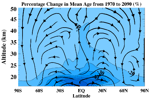
Figure 1. This figure shows the percentage change in mean age in the GEOSCCM from 1970 to 2090 and the change circulation (shown in black streamlines). The negative values indicate the mean age is getting younger as the circulation is speeding up. The largest percentage changes (approaching -50%) are in the tropical lower stratosphere.

Investigation of Stratospheric Water Vapor

Water vapor is a vitally important gas in our atmosphere. In the stratosphere, the region from 8-30 miles above the surface, water vapor plays a fundamental role both radiatively and chemically in Earth's climate system. Its stratospheric concentrations are principally controlled by changes in temperatures at the tropical tropopause, the lower boundary of the stratosphere, and changes in methane, which breaks down to form water vapor. Observations of past and model predictions of future water vapor changes are critically important for addressing many science issues, including the recovery of the ozone layer.

A recent paper by scientists at Johns Hopkins University and NASA's Goddard Space Flight Center (GSFC) used an advanced chemistry climate model to examine stratospheric water vapor trends and the factors that influence this trend. This work deconstructs the components that determine stratospheric water vapor concentrations so that the dominant impacts, which can change over space and time, can be understood. It was found that while significant warming occurs in the upper troposphere there was significant cooling happening in the lower stratosphere. This atmospheric balancing act results in much smaller temperatures changes near the critical tropical tropopause. Over the past 60 years and into the next 40 years the modeling results indicate that the break down of increasing methane concentrations will dominate stratospheric trends of increasing water vapor.

This study, which is part of a larger chemistry climate project at GSFC, examines just one component - stratospheric water vapor - in a highly coupled system, in which significant changes in water vapor can generate large changes throughout the climate system. Using a combination of observations and computer modeling this project seeks to improve our knowledge of Earth's climate system.

Citation:
Oman, L., D.W. Waugh, S. Pawson, R.S. Stolarski, and J.E. Nielsen, 2008. Understanding the Changes of Stratospheric Water Vapor in Coupled Chemistry-Climate Model Simulations. J. Atmos. Sci., 65, 3278-3291, DOI: 10.1175/2008JAS2696.1.

water_vapor Figure 1

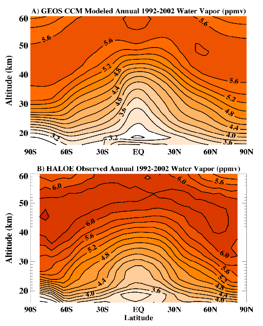
Figure 1. This figure shows the a) GEOSCCM modeled stratospheric water vapor concentrations (in ppmv, parts per million volume) compared to b) HALOE observed water vapor (ppmv) for 1992-2002. The model does a good job reproducing the mean stratospheric water vapor with only a small dry bias of about 0.4 ppmv.

The Impact of Very-Short-Lived Bromocarbons on Atmospheric Ozone

Proposal selected by ROSES-2010 A.14, Atmospheric Composition: Modeling and Analysis Program
PI: Qing Liang

Proposal Summary

We propose a 3-year project to investigate the impact of very-short-lived (VSL) bromocarbons on atmospheric ozone. The proposed project will be a multi-platform analysis that integrates the NASA Goddard GEOS Chemistry Climate Model (GEOSCCM) with satellite and suborbital data sets as well as ground and balloon measurements. Our objectives are:

To improve the understanding of oceanic emissions, transport, wet deposition of VSL bromocarbons and their products.
To develop climatology of the tropospheric and stratospheric BrO column
To quantify the impact of VSL bromocarbons on stratospheric ozone, current and future.

We will use aircraft measurements from NASA led field missions in PEM-Tropics, TRACE-P, INTEX, ARCTAS, TC4, AVE, and Pre-AVE to optimize oceanic emissions of very-short-lived (VSL) bromocarbons. We will use BrO measured by the balloon-borne LPMA/DOAS spectrometers, ground-based UV-visible, the AURA-OMI sensor to assess and improve atmospheric processes of bromine chemistry, transport, and deposition in GEOSCCM. We will use the simulated BrO and satellite BrO measurements from OMI to examine the spatial and temporal variability of BrO column and develop climatology of stratospheric and tropospheric BrO column for model and satellite validation. We will estimate the impact of VSL bromocarbons on stratospheric ozone since the 1960's. We will project GEOSCCM simulations into future (2010-2100) to calculate responses in ozone due to changes in ocean emissions, transport, ozone depleting substances and to establish a quantitative link between these driving mechanisms.

The proposed investigation is directly responsive to the ACMAP research elements described in ROSES 2010 A.14, Area C, utilizing observations to understand the impact of very short-lived halogen-containing species on the stratospheric halogen and ozone budgets.

Global modeling of nitrate and ammonium at present day and the year 2050: Implications for atmospheric radiation, chemistry, and ecosystems

PI: Huisheng Bian
Co-Is: Mian Chin, Xiaohua Pan, and Hongbin Yu
Collaborators: Bryan Duncan, Swen Metzger, Steven Pawson, and Jose Rodriguez

This MAP study investigates tropospheric nitrate and ammonium aerosols and their influence on atmospheric chemistry fields, radiative fields, and various ecosystems using NASA Global Modeling Initiative (GMI).

Nitrate and ammonium can influence air quality and ecosystems substantially, and their importance will be increasing in the future due to the predicted increase of ammonia emissions. However, there have been relatively few studies of nitrate and ammonium and the uncertainty of their representations in models is necessarily large.

Tasks proposed in this study are:

We will add seasonal information to the GEIA annual ammonia inventory. This is important since nitrate aerosol mostly forms in winter when it is cold.
We will implement a thermodynamic equilibrium model to partition semi-volatile species such as HNO3 between gas and aerosol phases. The simulated nitrate and ammonium aerosol will be evaluated using ground network measurements (CASTNET, EMEP, etc).
We will investigate the changes of atmospheric chemistry fields due to inclusion of nitrate and ammonium, which operate by altering the lifetime of nitric acid gas, providing additional particle surfaces for heterogeneous reactions, and changing photolysis rates. The simulated chemical fields of O3, NO2, and HNO3 will be evaluated using aircraft and satellite measurements including OMI and TES.
We will investigate the impact of nitrate particles on atmospheric radiative forcing using a NASA GSFC radiative transfer model (CLDRAD) and compare the results with estimates from other models.
We will use MODIS global characterization of landscapes and vegetation types together with our model results to estimate the nitrogen (including NOx, N2O5, NH3, HNO3, HO2NO2, NH4+, NO3-, PAN, and other organic nitrates) deposition to different ecosystems. A map of nitrogen "critical load", which is a deposition threshold above which detrimental impact may occur, will be summarized for ecosystems based on the available measurements. This provides a first order usage of our nitrogen deposition estimation.

Overall, the work will lead to a more complete treatment of the nitrate and ammonium aerosol lifecycle--from sources to chemical evolution and atmospheric impacts during transport to their ultimate fate and the subsequent potential effect on land and ocean ecosystems.

Improvements in Aerosol Microphysics, Radiation, and Chemical Interaction in the GEOS Chemistry-Climate Model: Applications to Atmospheric Brown Clouds

PI: Peter Colarco

In this proposal we will improve our understanding of the composition, microphysics, and radiative properties of atmospheric aerosols in simulations of the aerosols in the polluted regions in India and southeast Asia, where the so-called atmospheric brown clouds strongly impact regional dynamics and air quality. We will additionally investigate the interaction of aerosols and tropospheric chemistry. Our approach will be to:

introduce an online core-shell radiation code for calculation of the optical properties of internally mixed aerosols
develop offline lookup tables of aerosol optical properties for non-spherical, inhomogeneous aerosols
constrain simulated aerosol composition and optical properties with regional datasets
investigate the impact of improved treatment of aerosol composition and optics on atmospheric heating rates and chemical photolysis rates
investigate the interaction of running online aerosols and chemistry together

We will initially focus on present-day (1999-2010) conditions with driven by the Modern-Era Retrospective-analysis for Research and Applications (MERRA) reanalysis data. Our objective is to realistically simulate aerosol distributions and composition as determined by comparisons to satellite (e.g., OMI, MODIS, MISR, CALIPSO) sensors and ground-based (e.g., AERONET) observations, in particular leveraging on our involvement in the ongoing TIGERZ campaign. With our model constrained by the previous experiments, we will perform climate simulations of present-day and mid-century (2041 - 2050) aerosol distributions and composition. Our objective is to deconvolve the impact of aerosol composition on regional climate from the impacts of changes in tropospheric chemistry, sea surface temperatures, and greenhouse gas concentrations.