Atmospheric Chemistry and Dynamics Laboratory (Code 614)
For Our Colleagues Scientific/Technical Information

The Quasi-biennial Oscillation (QBO)
This web page shows the Quasi-biennial Oscillation (QBO) near real-time and historical behavior over the satellite-era (1980–present). Daily plots are updated at least once per day, while monthly plots are updated on the 2nd day of the following momth.
Current QBO condition
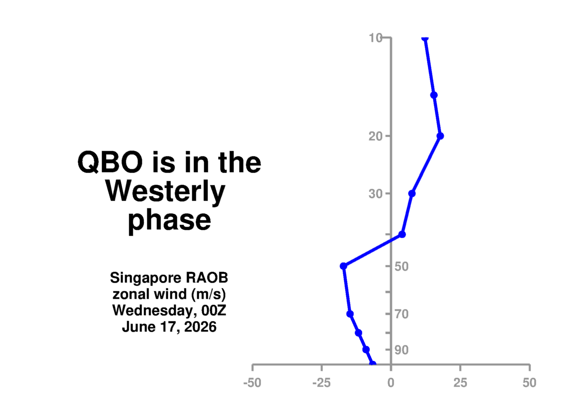
Table of Contents
- Introduction
- Zonal wind plots
- Singapore sonde u-wind versus pressure
- Equator MERRA-2 u-wind versus pressure
- Singapore last 3 years' u-wind versus pressure
- MERRA-2 u-wind versus latitude
- MERRA-2 u-wind versus latitude and pressure
- Singapore EOF 1 and 2 zonal wind pattern
- Temperature plots
- Singapore sonde T versus pressure (deseasonalized)
- Equator MERRA-2 T versus pressure (deseasonalized)
- Singapore last 3 years' T versus pressure
- MERRA-2 T versus latitude (deseasonalized)
- MERRA-2 Temperature versus latitude and pressure
- Vertical velocity (W*) plots
- Equator (5S-5N) MERRA-2 W* versus pressure (deseasonalized)
- MERRA-2 W* versus latitude (deseasonalized)
- Zonal mean wind momentum budget
- Ozone plots
- Total ozone from TOMS/OMI versus latitude (deseasonalized)
- Daily total ozone from TOMS/OMI versus latitude (deseasonalized)
- MLS Ozone versus pressure (deseasonalized)
- MLS Ozone versus Latitude (deseasonalized)
- Water plots
- QBO movie
- Data links
- External links
Introduction
The Quasi-biennial Oscillation (QBO) is a tropical, lower stratospheric, downward propagating zonal wind variation, with an average period of ~28 months. The importance of the QBO is that it dominates the variability of the tropical lower stratospheric meteorology [Wallace, 1973]. The QBO is also important for seasonal forecasting, and the QBO controls stratospheric ozone and water variability that can modulate surface ultra-violet (UV) and infrared (IR) radiation.
Ebdon [1960] and Reed et al. [1961] independently first detected the QBO in the early 1960s. Tropical radiosonde wind observations that document the QBO have been made continuously since 1953 [e.g., Naujokat, 1986], and these early observations are available at the Freie Universität of Berlin.
A comprehesive QBO summary (with a description of the cause of the QBO) can be found in Baldwin et al. [2001].Data herein are from radiosondes, NASA GSFC/GMAO assimilated data, and NASA satellites. The radiosondes are from the Meteorological Service Singapore Upper Air Observatory (station code 48698). The station is located at 1.34041N, 103.888E at an altitude of 21m.
The assimilated data are from the Modern-Era Retrospective analysis for Research and Applications, Version-2 (MERRA-2). MERRA-2 provides data beginning in 1980 and runs a few weeks behind real time [Gelaro et al., 2017]. The structure, dynamics, and ozone for the QBO in MERRA-2 is documented in Coy et al. [2016].
These plots also reveal the QBO disruption that occured from late 2015 through about February 2017 [Newman et al., 2016; Osprey et al., 2017]. A more complete dynamical explanation of the disruption can be found in Coy et al. [2017] with another paper describing the deceleration as being caused by a very strong wave packet Lin et al. [2019]. The impact on ozone, water, etc., can be found in Tweedy et al. [2017].
Zonal winds
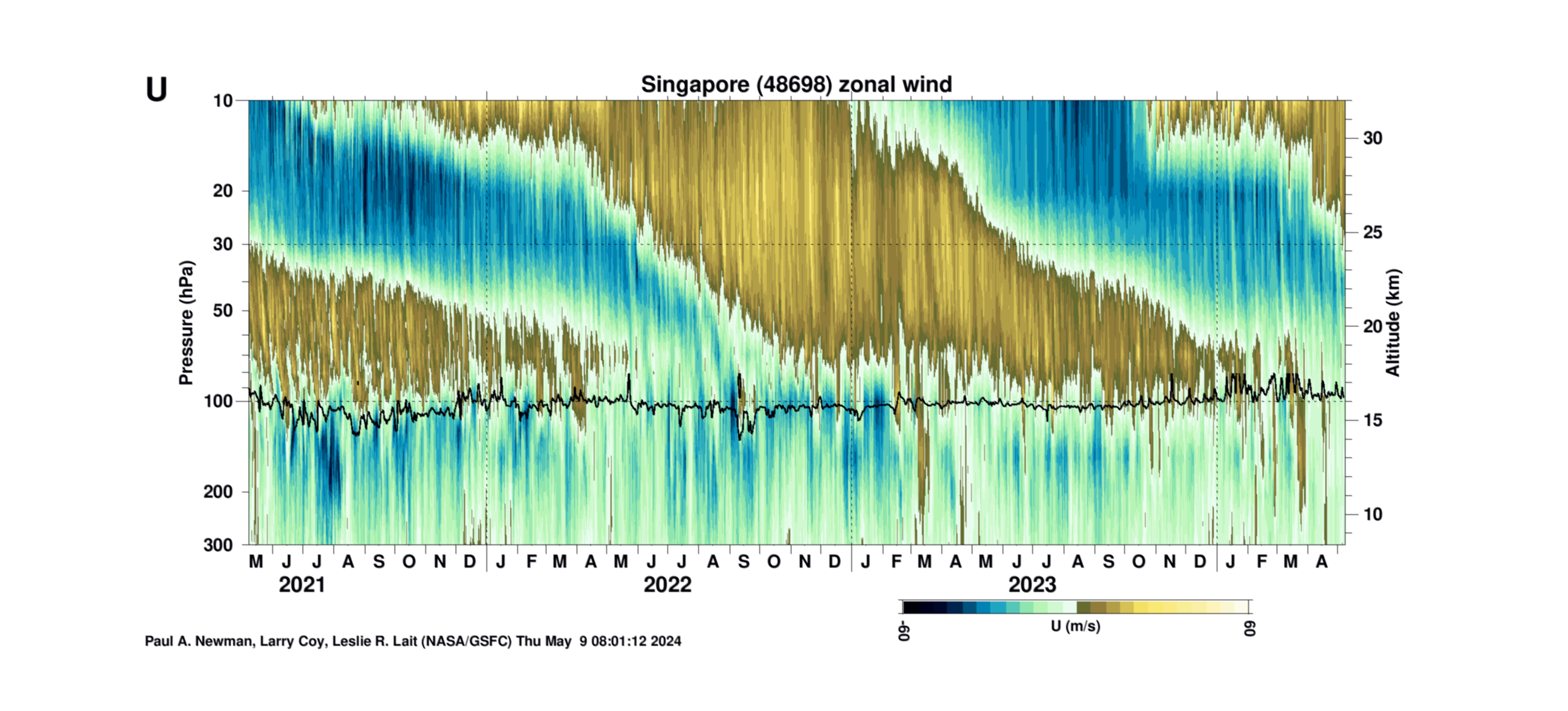
Singapore sonde 1980–present QBO from monthly mean zonal wind
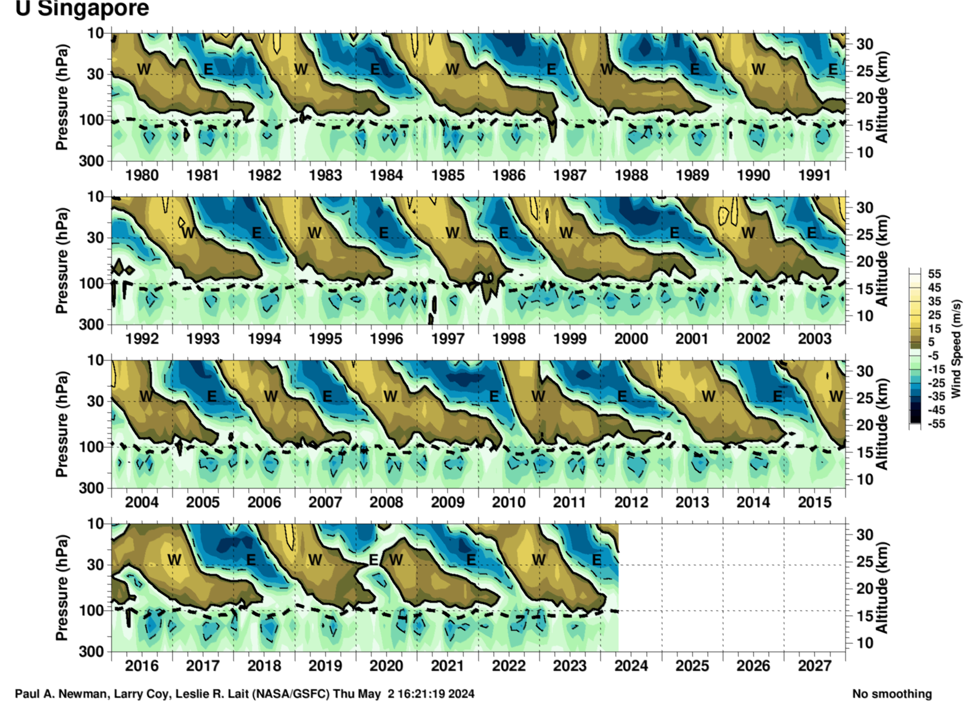
The plot is made by: 1) reading all daily sondes for the full month (generally twice per day at 0Z and 12Z), 2) vertically interpolating the zonal wind to missing levels (no extrapolation to levels above balloon burst altitudes), and 3) time interpolating for missing levels above the top of the balloon profile. The thick dotted line shows the tropopause calculated from the thermal lapse rate. Units are meters per second.
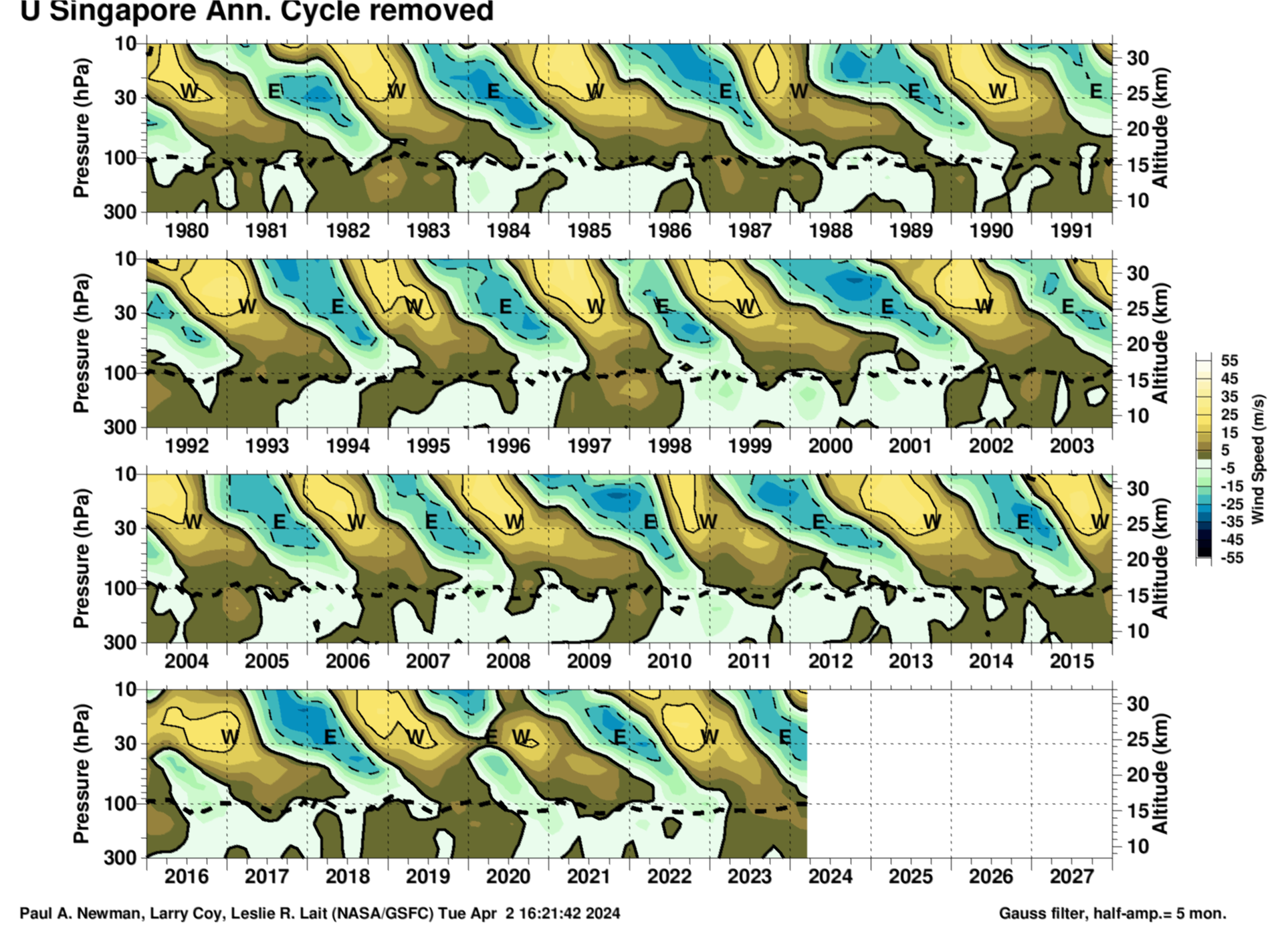
As above, but with annual cycle removed and a 5-month Gaussian smoothing (png), (high-res PDF).
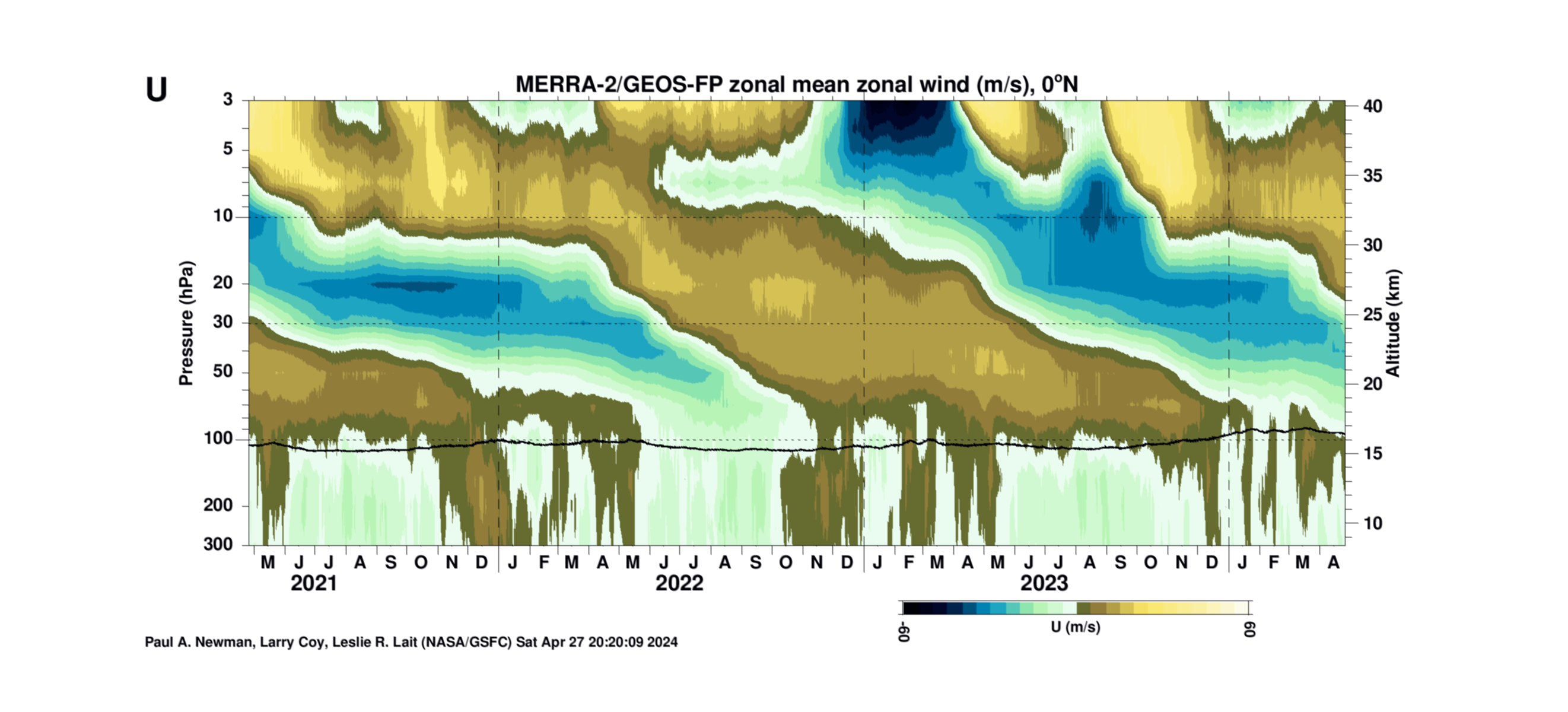
MERRA-2 1980–present QBO monthly mean zonal wind at the Equator
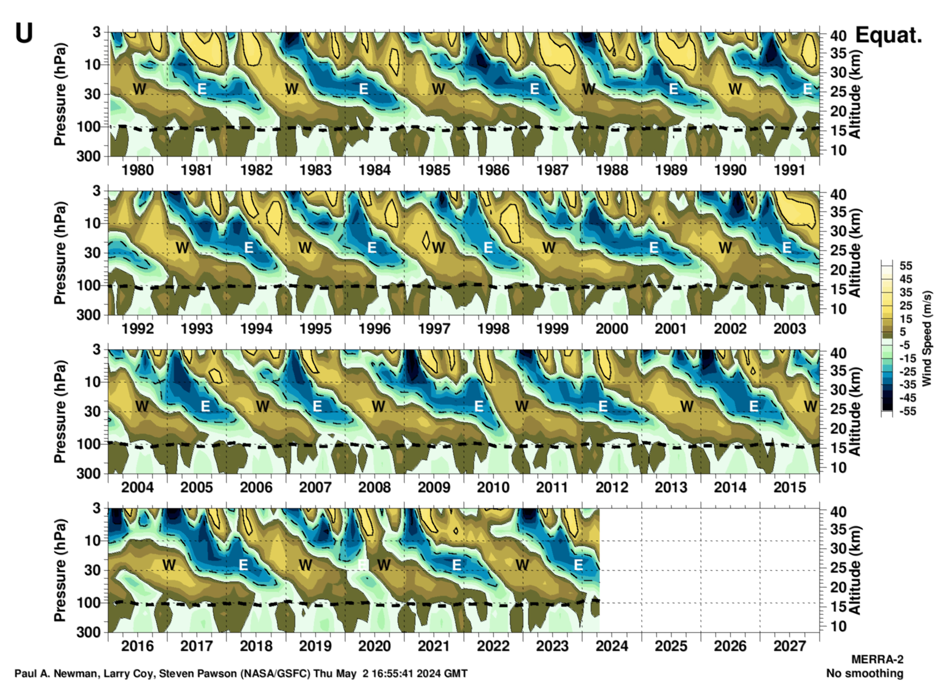
The plot is generated from the monthly mean MERRA-2 zonal mean winds. The thick dotted line shows the tropopause calculated from the thermal lapse rate. The noted easterly (E) and westerly (W) phases are derived from the Singapore sonde above. Units are meters per second.
MERRA-2 zonal wind plot as above(png) (high-res PDF), but winds are detrended and the annual cycle removed.
The last 3 years of the QBO from the Singapore sonde daily zonal wind
The plot shows the daily zonal mean winds from the twice per day (0Z and 12Z) Singapore radiosondes. Each sonde is interpolated to a 0.5 km vertical grid. Above the burst altitude, either MERRA-2 or GEOS-FP data are used to fill this vertical grid. The black line shows the tropopause as computed from the lapse rate. Units are meters per second.
As above, but MERRA-2 zonal mean equatorial wind to 3 hPa (PDF, png. ).
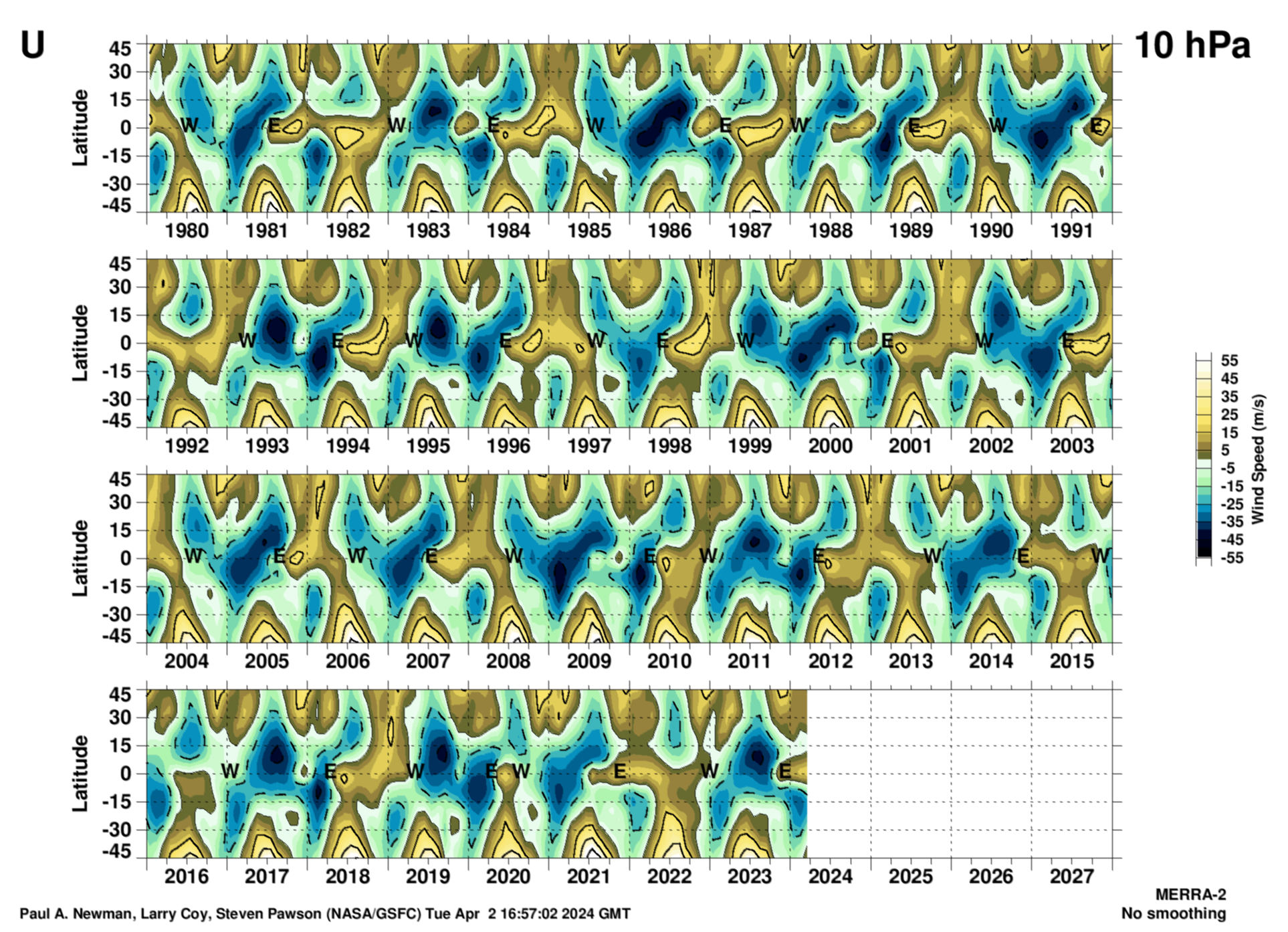
MERRA-2 1980–present QBO monthly mean zonal wind versus latitude
These plots show how the QBO phase connects to midlatitude, midwinter westerlies.
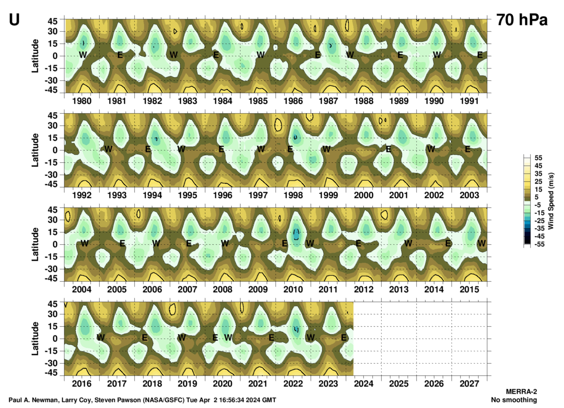
70 hPa
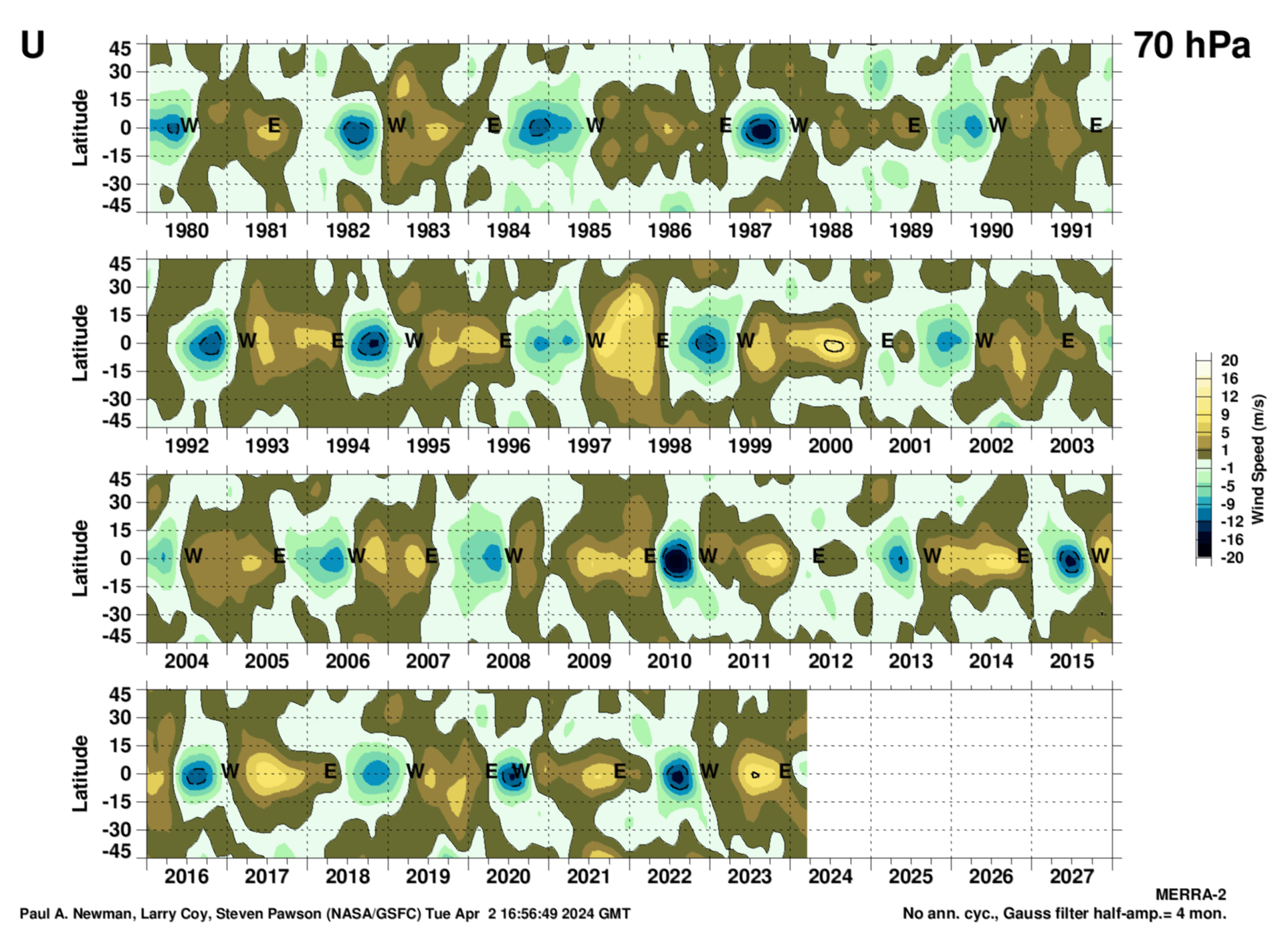
The latitudinal structure of the zonal mean wind QBO from MERRA-2 at 70 hPa. These data have had the annual cycle removed to reveal the QBO. Units are meters per second.
Zonal mean wind that INCLUDEs the annual cycle High-res PDF version (png). Units are meters per second.
40 hPa
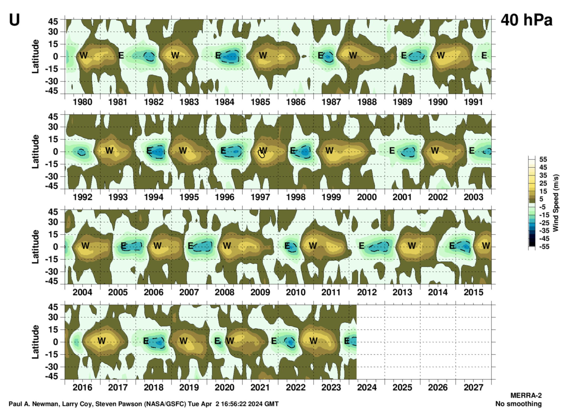
The latitudinal structure of the zonal mean wind QBO from MERRA-2 at 40 hPa. These data have had the annual cycle removed to reveal the QBO. Units are meters per second.
Zonal mean wind that INCLUDEs the annual cycle High-res PDF version (png). Units are meters per second.
10 hPa
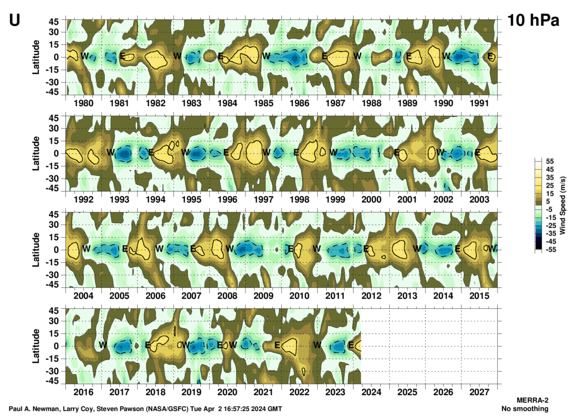
The latitudinal structure of the zonal mean wind QBO from MERRA-2 at 10 hPa. These data have had the annual cycle removed to reveal the QBO. Units are meters per second.
Zonal mean wind that INCLUDEs the annual cycle High-res PDF version (png). Units are meters per second.
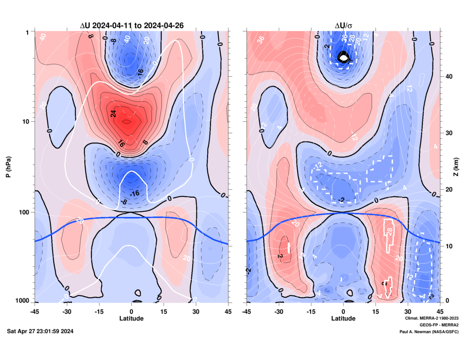
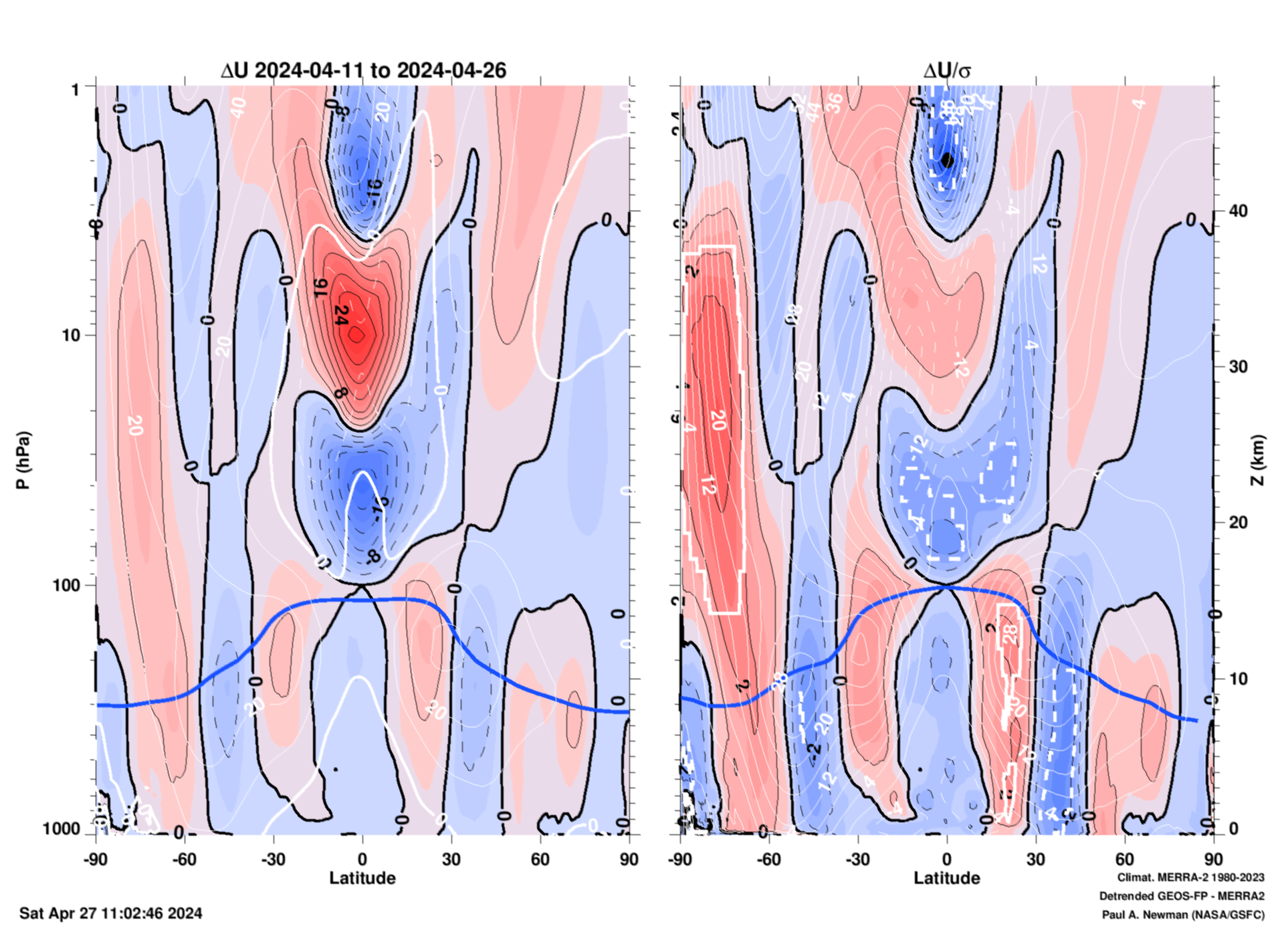
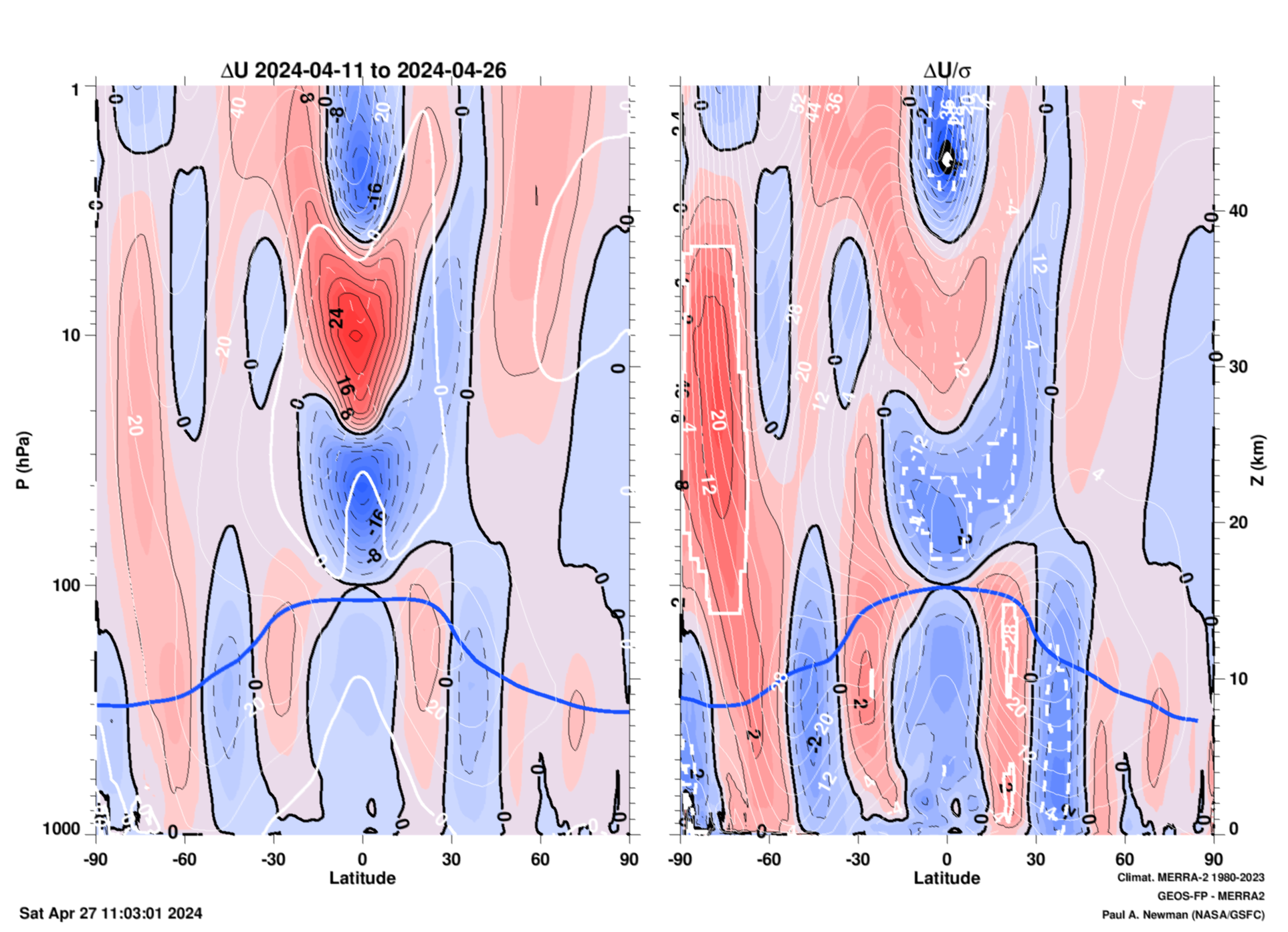
QBO zonal mean zonal wind (\(\overline u\)) latitude vs. pressure for the last 15 days.
The plot is made by time averaging the 12Z GEOS-FP zonal mean analyses for the last 15 days. The 1980–2022 MERRA-2 climatological average for these same 15 days is subtracted from the current 15-day average. Hence, the annual cycle is removed. The data are also detrended to show QBO effects, not climate effects.
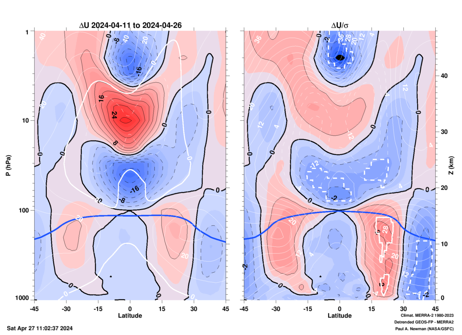
Left panel: Wind anomlies (\(\Delta \overline u \) = \(\overline u\) - <\(\overline u \)>, where overbars are zonal means, and brackets are multi-year averages. Positive anomalies are red and negative anomalies are blue (units = m/s). The white lines show the wind climatology and the thick blue line is the climatological tropopause (computed from the Brunt-Vaisalla frequency). The left y-axis is pressure (hPa), and the right y-axis is pressure altitude (km). Right panel: Normalized wind anomalies (\(\Delta \overline u/\sigma \)). \(\sigma \) (the multi-year time series' standard deviation) is calculated from the same 15-day periods over the 43 years 1980–2022 MERRA-2 climatology. As an example, values of of \(\Delta \overline u/\sigma = 2 \) are two standard deviations above the norm. The (solid and dashed) thick white lines on this RHS indicate record (positive and negative) anomaly values. The actual anomaly values are plotted as the thin white lines.
Same 45°S–455°N zonal wind anomalies but the trend is NOT removed (pdf, png).
Same zonal wind anomalies as above with the trend removed, but for 90°S–90°N (pdf, png). And without the trend removed (pdf, png).
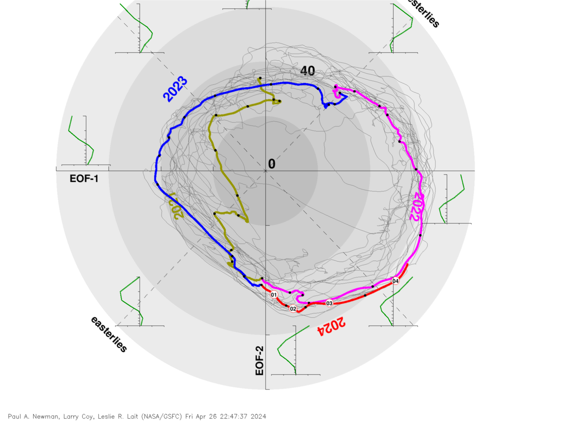
The EOFs of the 1980–present QBO from the Singapore sonde monthly mean winds
The empirical orthogonal functions (EOFs) of the Singapore winds represent the major components of the QBO's variability. The EOFs are calculated following [Wallace et al., 1993]. The EOFs were derived from the 1979–present deaseasonalized monthly mean Singapore radiosonde zonal winds (shown above) using 100–10 hPa zonal winds. The first two EOFs show the circular polarization that is characteristic of the QBO in the counter-clockwise rotation. On the rim of the figure are the simple reconstructuions of the zonal wind profile for the various phases. The last 3 calendar years are colored. This plot was shown in Tweedy et al. [2017]. Units are meters per second.
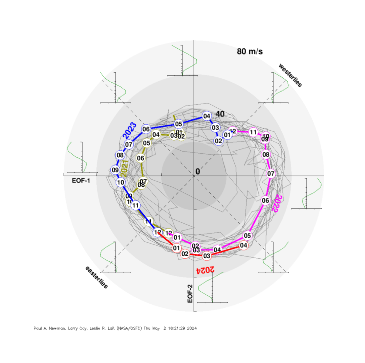
Phase diagram of the first two leading modes of the calculated EOFs from the Singapore winds shown above. On the rim of the figure are the simple reconstructions of the zonal wind profile for the various phases. The last 3 calendar years are colored. Circles indicate the month number for the corresponding year.
As above, but from MERRA-2/GEOS-FP zonal mean zonal equatorial winds (PDF, and png).. These data are smoothed using a 10-day half-amplitude Gaussian filter.
Temperatures
Singapore sonde temperature QBO from monthly mean averages
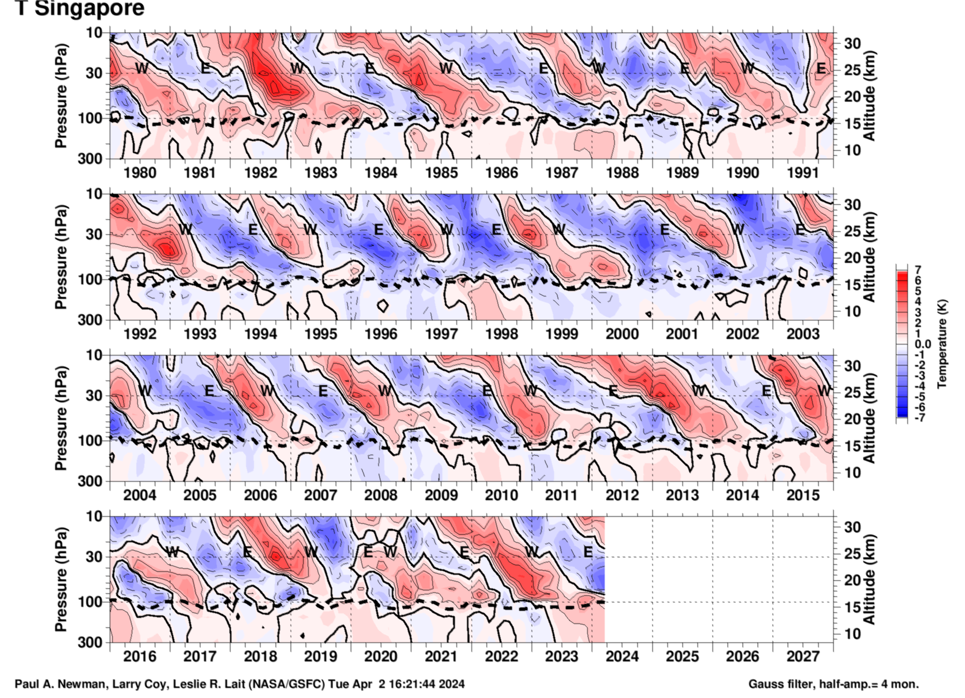
The plot is generated by: 1) reading in monthly mean temperatures, 2) detrending the temperature time series, 3) subtracting off the annual cycle at all levels, and 4) smoothing the data with a 1-2-1 Gaussian filter (effectively removing variability with periods of 5 months or less. The thick dotted line shows the tropopause calculated from the thermal lapse rate. Units are Kelvin.
MERRA-2 temperature QBO from monthly mean data at the Equator
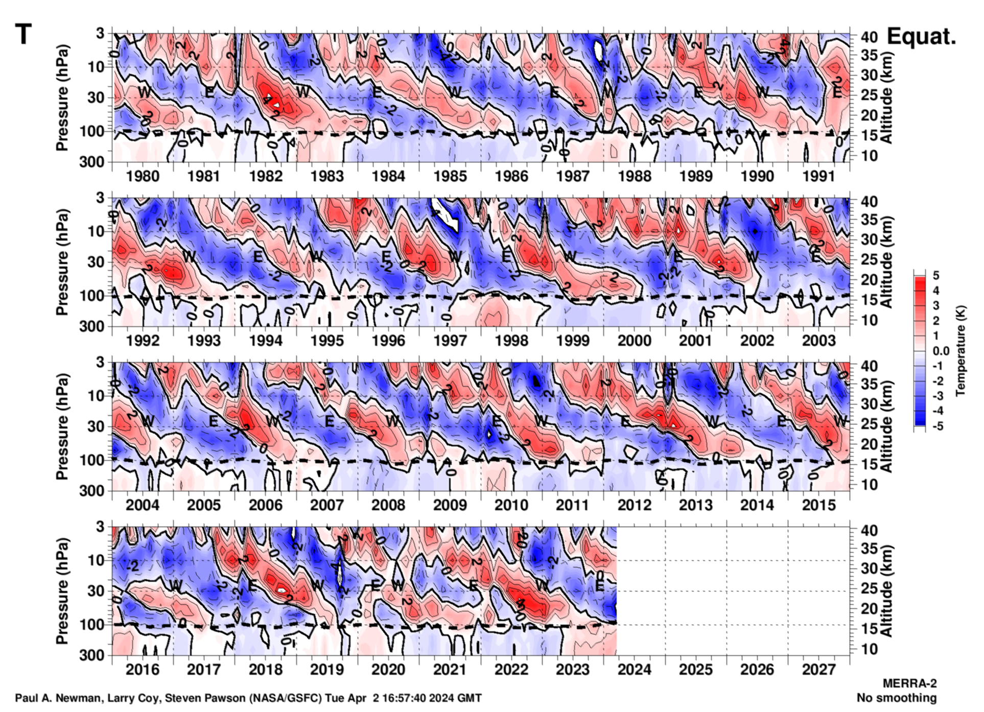
This temperature plot is generated by: 1) reading in the monthly mean MERRA-2 zonal mean temperature, 2) subtracting the long-term averaged monthly mean, and 3) performing a linear detrending of the residual temperature. The thick dotted line shows the tropopause calculated from the thermal lapse rate. Note that the QBO wind peaks tend to fall along the "zero" temperature lines. Units are Kelvin.
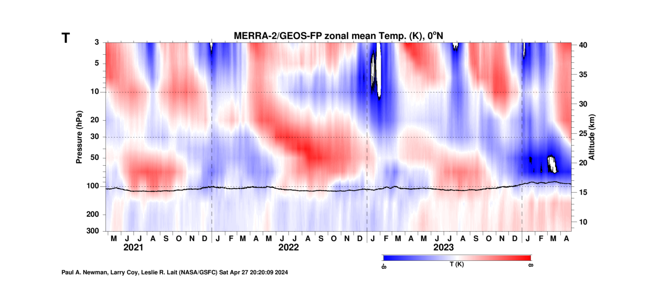
The last 3 years of the temperature QBO from the Singapore twice daily sondes

Daily zonal mean temperatures from the twice per day (0Z and 12Z) Singapore radiosondes. Each sonde is interpolated to a 0.5 km vertical grid. Above the burst altitude, either MERRA-2 or GEOS-FP data are used to fill this vertical grid. The 3-year time average profile is subtracted from the data (annual cycle is still embedded in the plot). The tropopause is shown as the black line (computed from the lapse rate). Units are Kelvin.
As above, but MERRA-2 zonal mean equatorial wind to 3 hPa (PDF, png. ).
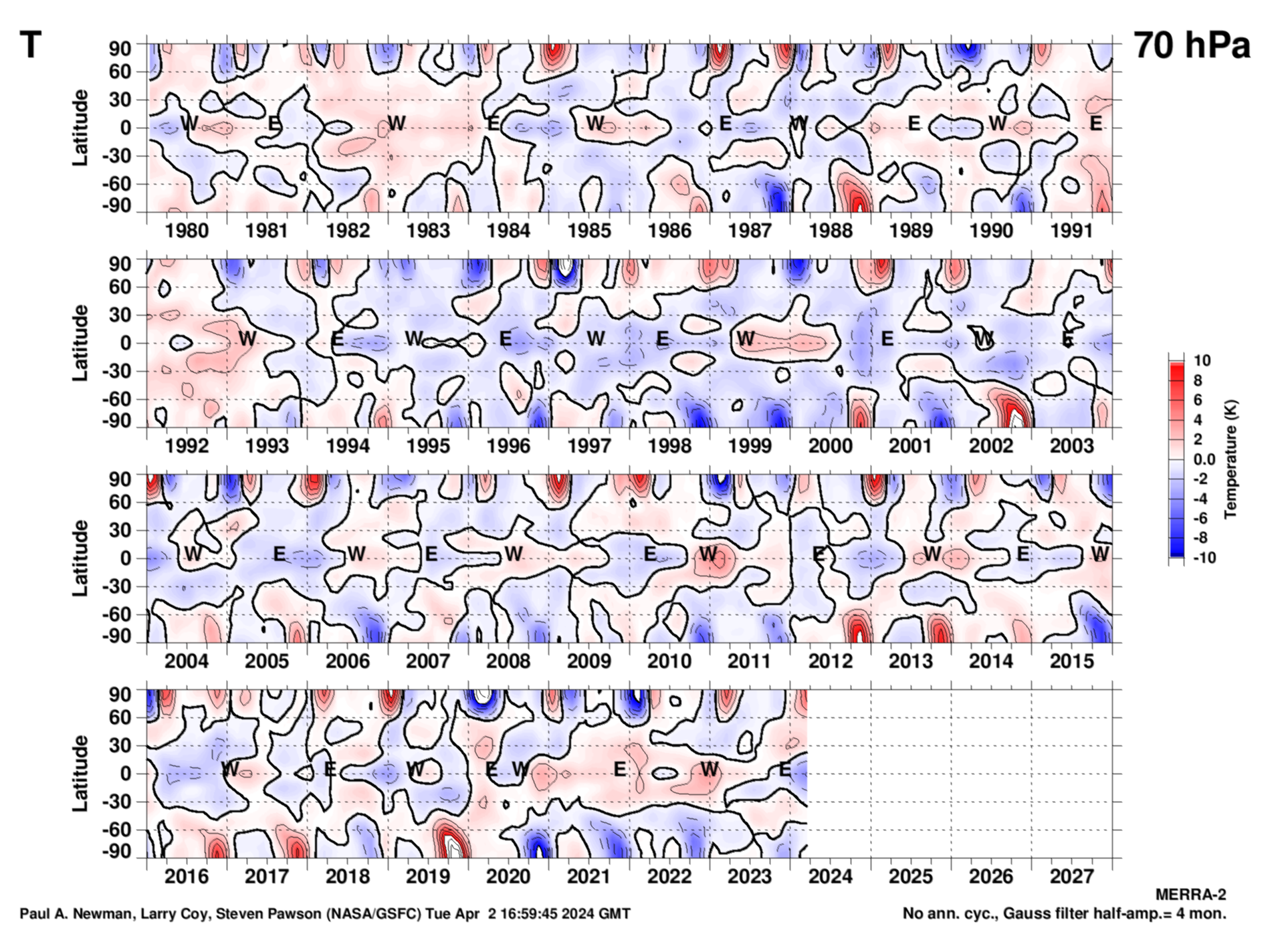
MERRA-2 temperature (deseasonalized) QBO from monthly mean data versus latitude
70 hPa
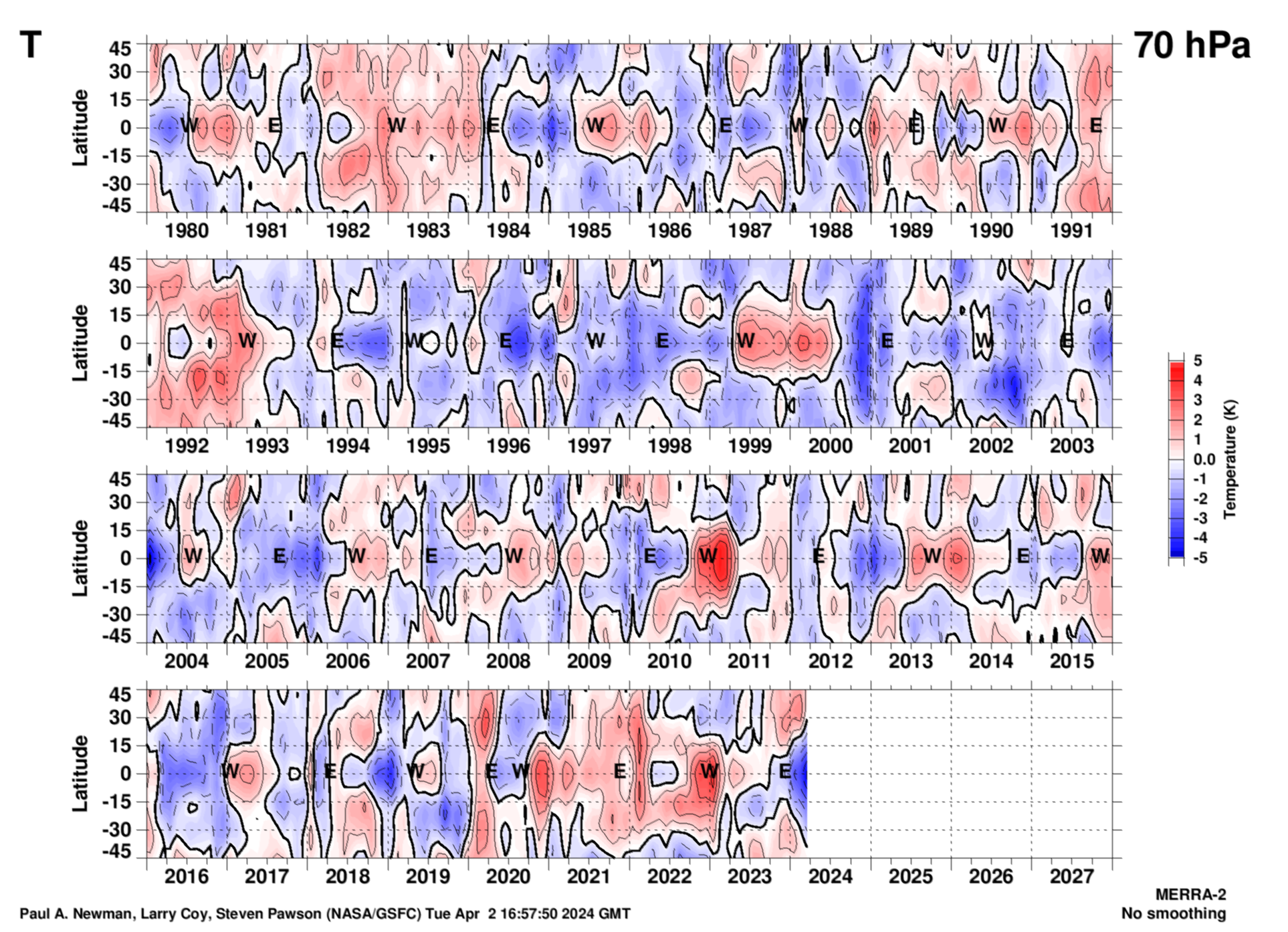
As with the zonal winds, this temperature plot is generated by taking the monthly mean MERRA-2 zonal mean temperatures, subtracting the long-term monthly mean, and then linearly detrending the residual temperature. The easterly (E) and westerly (W) points are from the Singapore zonal winds, and are defined by the EOF-1 and EOF-2 phase diagram above. Units are Kelvin.
Same plot, but 90°S–90°N high-res PDF (png).
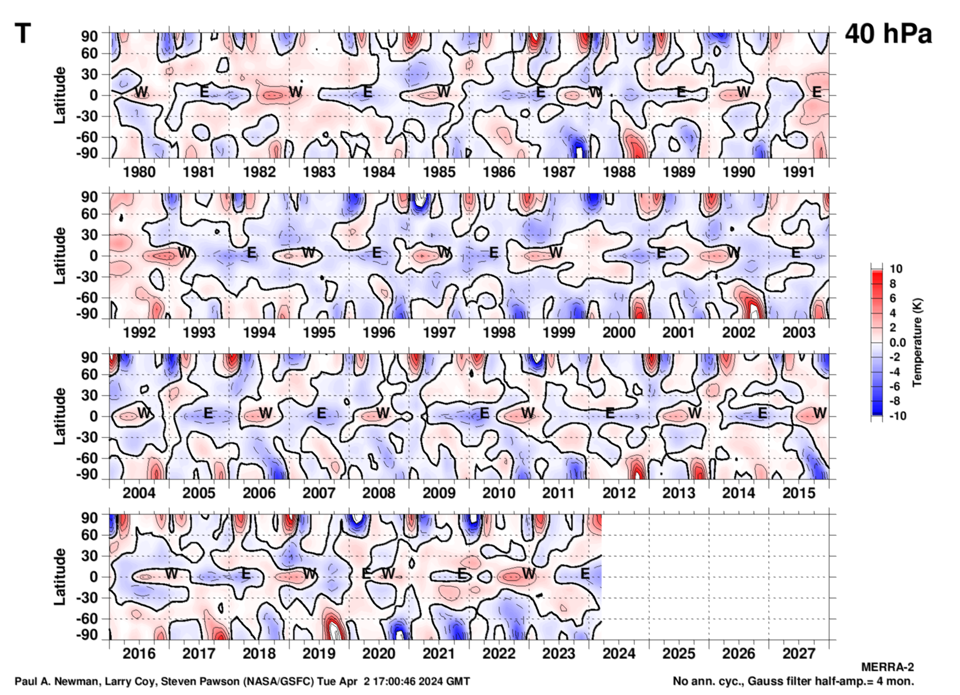
40 hPa

As with the zonal winds, this T plot is generated by taking the monthly mean MERRA-2 zonal mean temperatures, and then subtracting the long-term monthly mean, and then linearly detrending the residual temperature. The easterly (E) and westerly (W) points are from the Singapore zonal winds, and are defined by the EOF-1 and EOF-2 phase diagram above. Units are Kelvin.
Same plot, but 90°S–90°N high-res PDF (png).
10 hPa
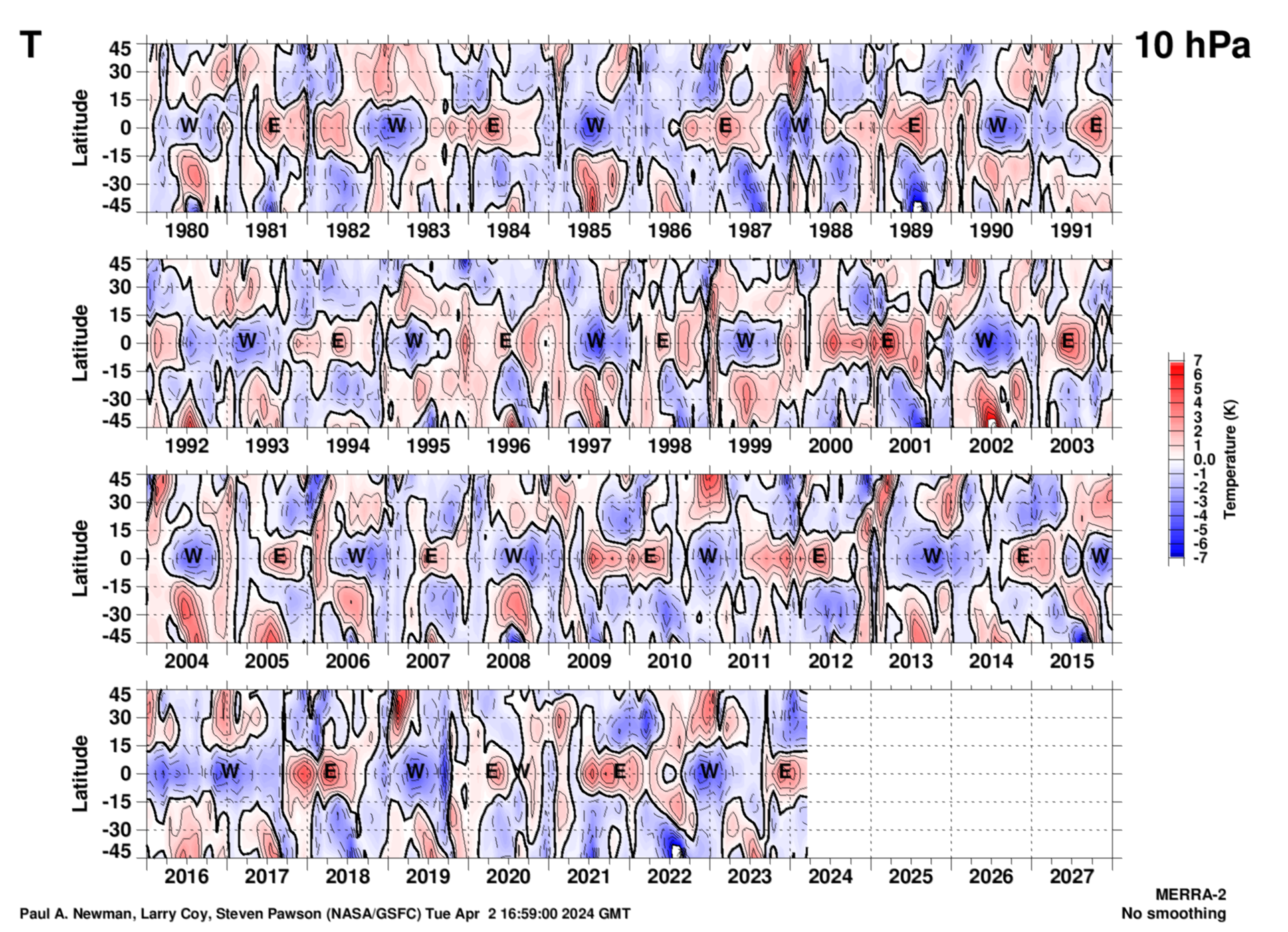
As with the zonal winds, this T plot is generated by taking the monthly mean MERRA-2 zonal mean temperatures, and then subtracting the long-term monthly mean, and then linearly detrending the residual temperature. The easterly (E) and westerly (W) points are from the Singapore zonal winds, and are defined by the EOF-1 and EOF-2 phase diagram above. Units are Kelvin.
Same plot, but 90°S-90°N high-res PDF (png).
QBO zonal mean temperature (\(\overline T\)) latitude vs. pressure for the last 15 days
The plot is made by time averaging the 12Z GEOS-FP zonal mean analyses for the last 15 days. The 1980–2022 MERRA-2 climatological average for these same 15 days is subtracted from the current 15-day average. Hence, the annual cycle is removed. The data are also detrended to show QBO effects, not climate effects.
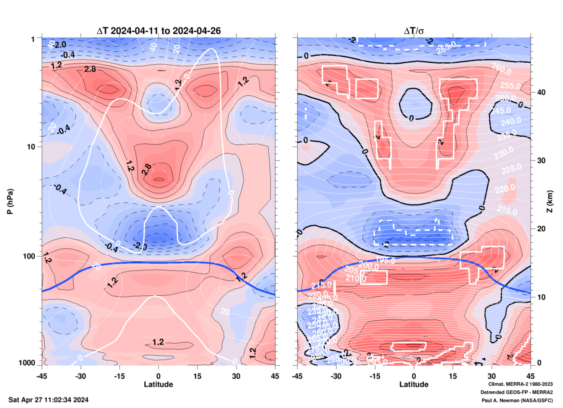
Left panel: Temperature anomlies (\(\Delta \overline T \) = \(\overline T\) - <\(\overline T \)>, where overbars are zonal means, and brackets are multi-year averages. Positive anomalies are red and negative anomalies are blue (units = K). The white lines show the \(\overline u\) wind climatology and the thick blue line is the climatological tropopause (computed from the Brunt-Vaisalla frequency). The left y-axis is pressure (hPa), and the right y-axis is pressure altitude (km). Right panel: Normalized temperature anomalies (\(\Delta \overline T/\sigma \)). The temperature standard deviation (\(\sigma \)) is calculated from the same 15-day periods over the 43 years 1980–2022 MERRA-2 climatology. As an example, values of of \(\Delta \overline T/\sigma = 2 \) are two standard deviations above the norm. The (solid and dashed) thick white lines on this RHS indicate record (positive and negative) anomaly values. The actual temperature values are plotted as the thin white lines.
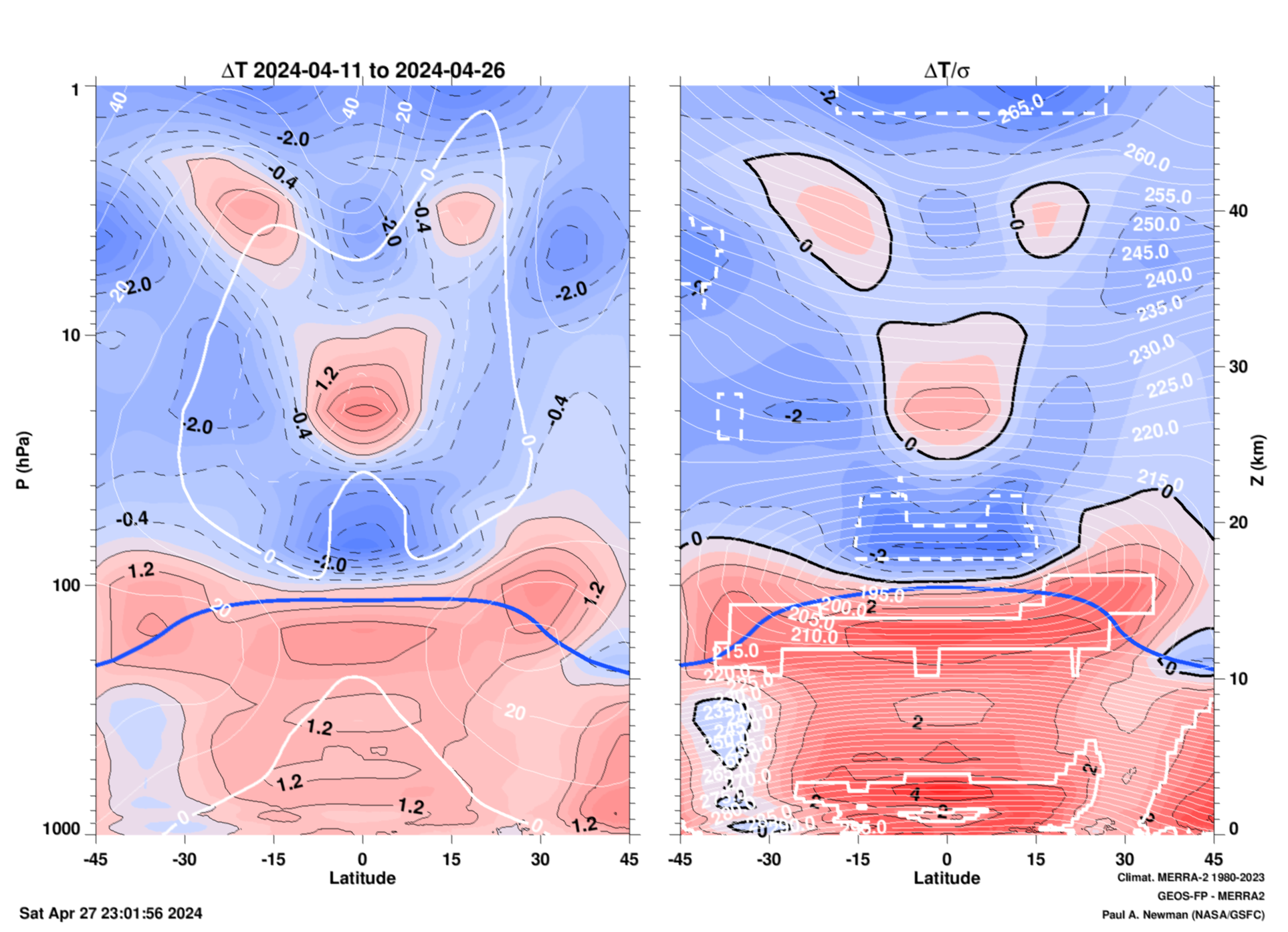
Same 45°S–45°N temperature anomalies but the trend is NOT removed (pdf, png).
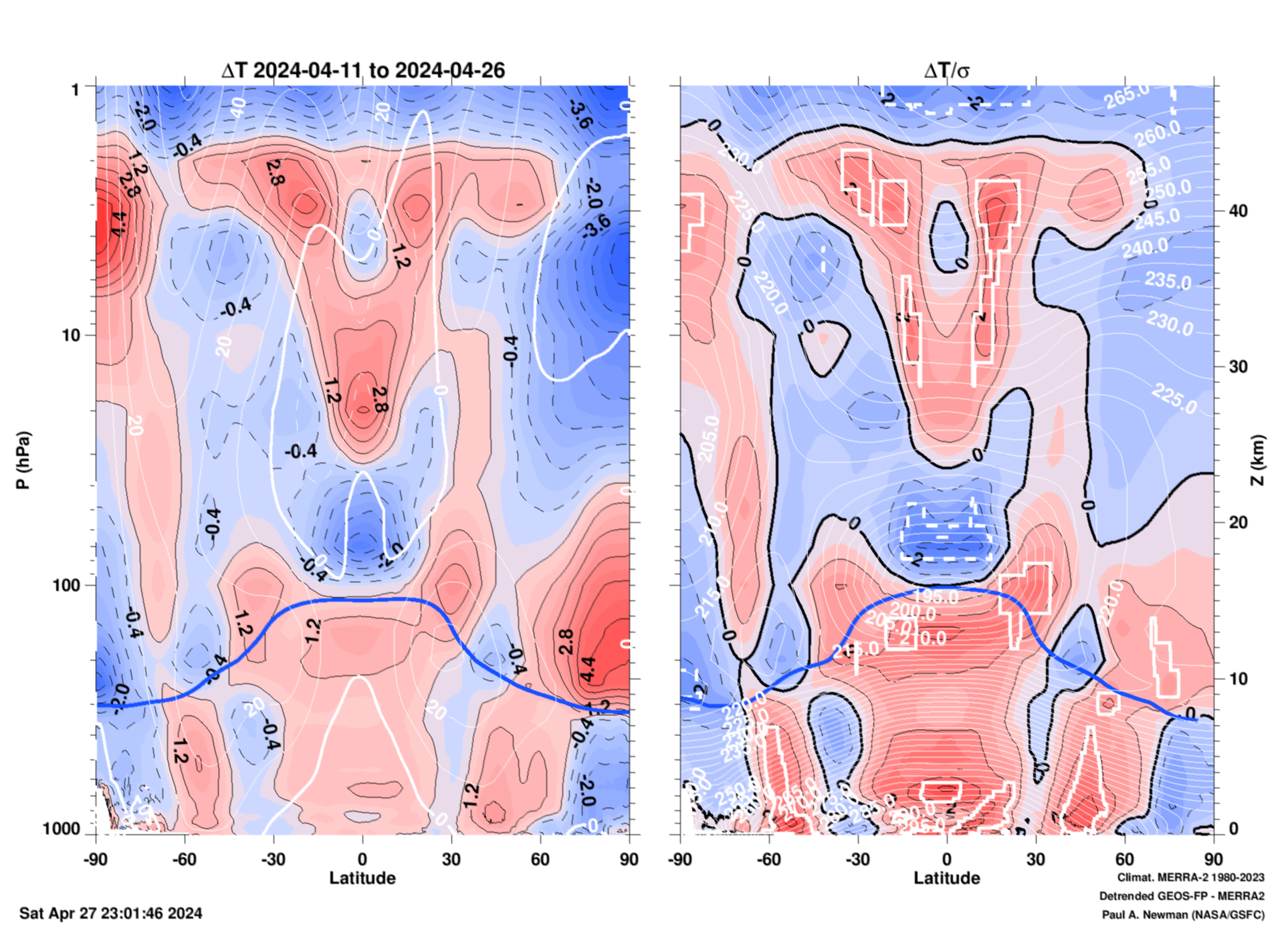
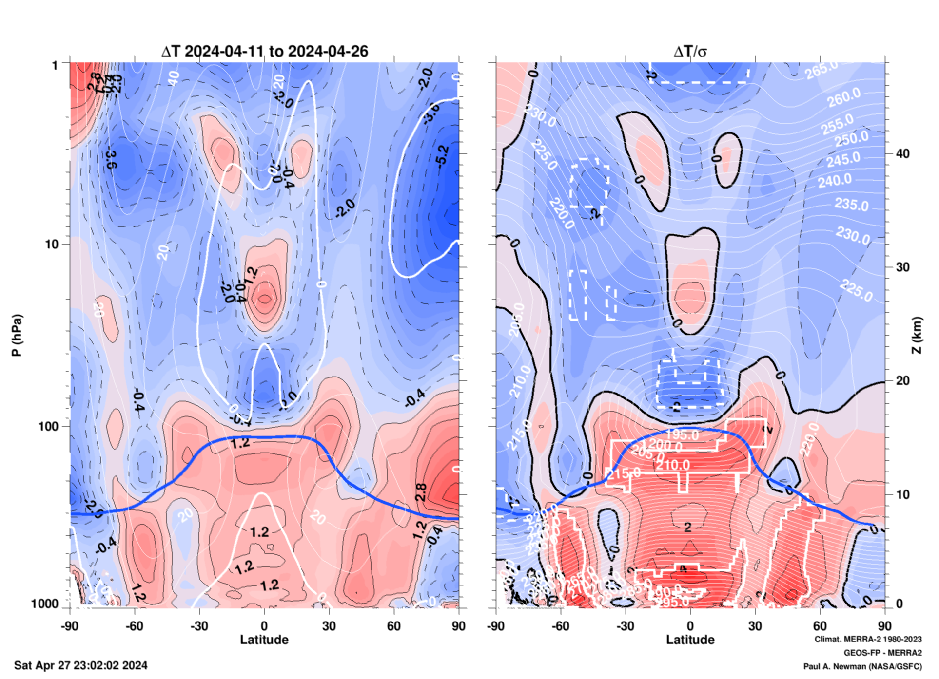
Same temperature anomalies as above with trend removed, but for 90°S-90°N (pdf, png). And without the trend removed (pdf, png).
Vertical residual velocity (\(\overline {w}^*\))
In the lower stratosphere, the QBO is anti-correlated with the vertical residual velocity. The normal lifting is enhaced in easterlies (E) and reduced in westerlies (W).
MERRA-2 \(\overline {w}^ *\) QBO from monthly mean data at the Equator (5S-5N)
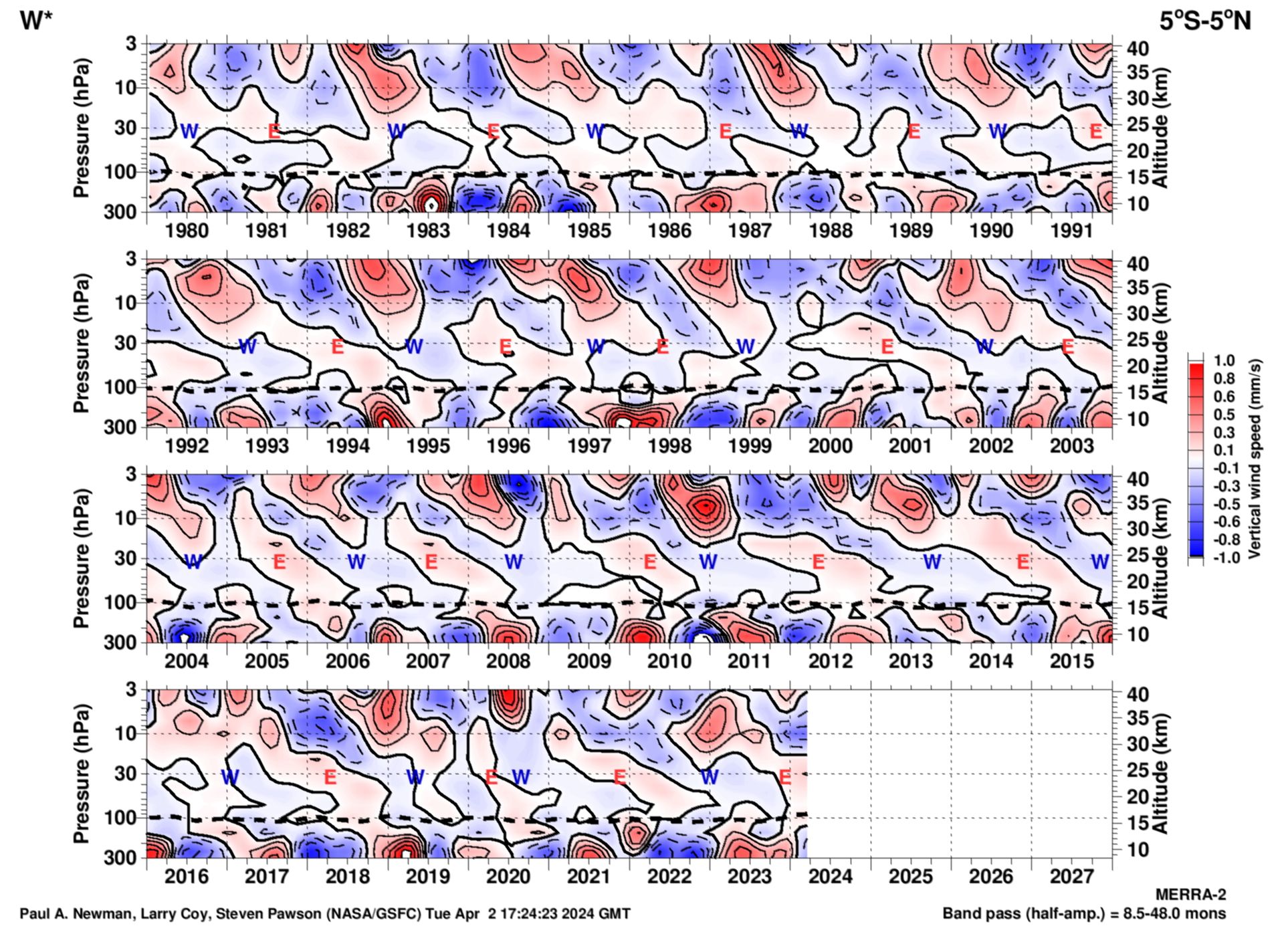
This \(\overline {w}^*\) plot is generated from MERRA-2 zonal mean values. The annual cycle and the linear trend of the 1980–present time series are both removed, and the values are band pass filtered with a Gaussian filter (8.5–48.0 months). The thick dotted line shows the tropopause calculated from the thermal lapse rate. The QBO is well correlated in the post-1999 period, but relatively poor prior to that date. This is probably related to the increased assimilation of satellite data in the post-1999 period.
MERRA-2 \(\overline {w}^*\) QBO from monthly mean data versus latitude
70 hPa
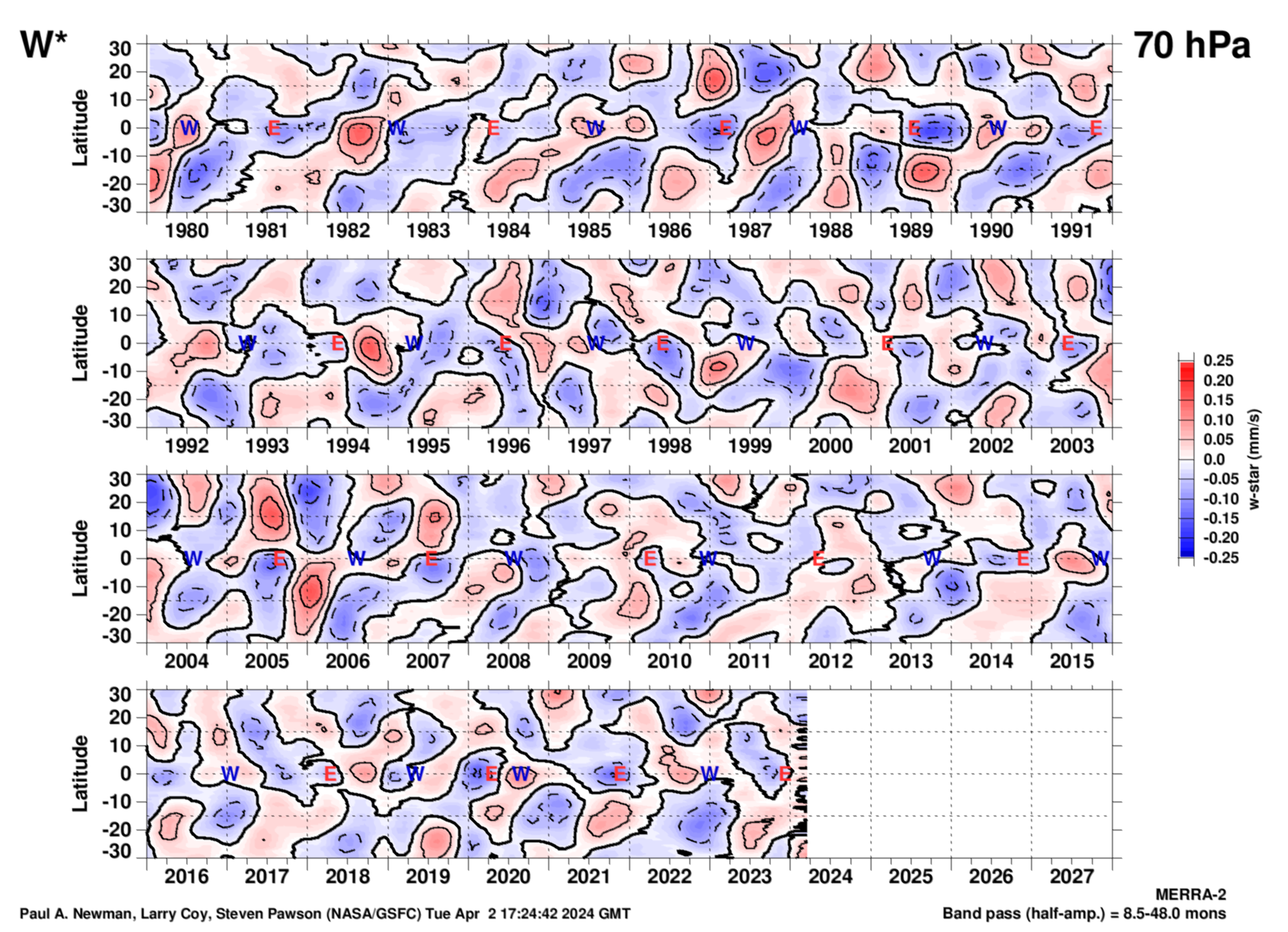
As with the zonal winds, this \(\overline {w}^*\) plot is generated from the monthly mean MERRA-2 zonal mean omega, heat flux, and temperature values. The long-term monthly means are subtacted, and then linearly detrended. The easterly (E) and westerly (W) points are from the Singapore zonal winds, and are defined by the EOF-1 and EOF-2 phase diagram above. Units are millimeters per second.
40 hPa
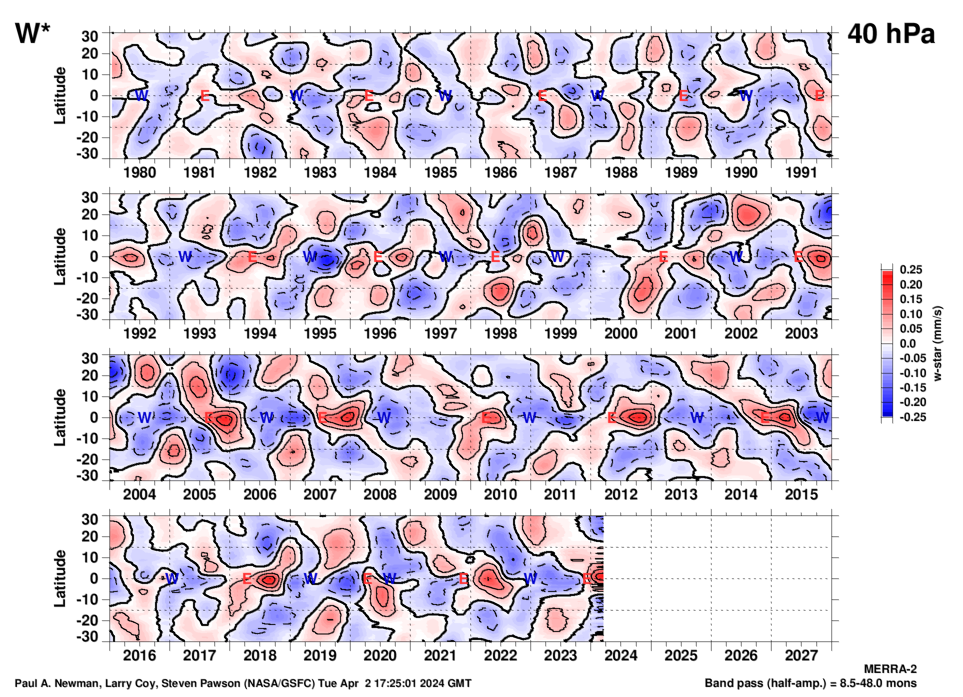
As with the zonal winds, this \(\overline {w}^*\) plot is generated from the monthly mean MERRA-2 zonal mean omega, heat flux, and temperature values. The long-term monthly means are subtacted, and then linearly detrended. The easterly (E) and westerly (W) points are from the Singapore zonal winds, and are defined by the EOF-1 and EOF-2 phase diagram above. Units are millimeters per second.
10 hPa
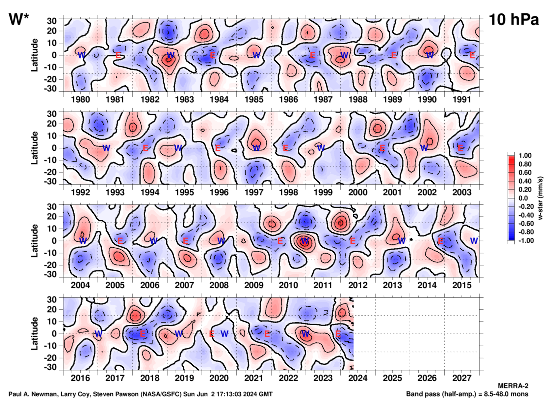
As with the zonal winds, this \(\overline {w}^*\) plot is generated from the monthly mean MERRA-2 zonal mean omega, heat flux, and temperature values. The long-term monthly means are subtacted, and then linearly detrended. The easterly (E) and westerly (W) points are from the Singapore zonal winds, and are defined by the EOF-1 and EOF-2 phase diagram above. Units are millimeters per second.
Zonal mean wind momentum budget
Ozone
Total ozone from TOMS/OMI series versus latitude (deseasonalized)
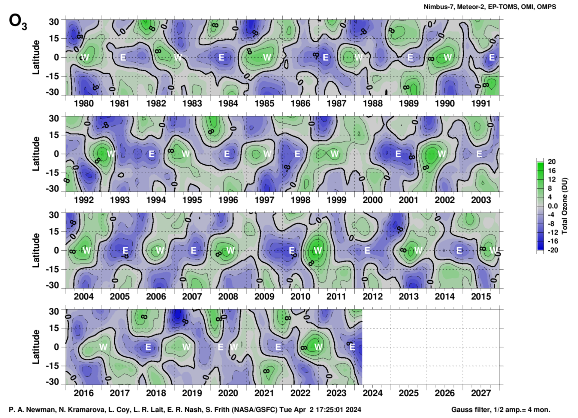
Total ozone monthly means versus latitude. The plot is generated by: 1) reading in monthly mean total ozone, 2) subtracting off the annual cycle at all levels, 3) detrending the total ozone time series with a linear term over the entire time series, and 4) smoothing the data with a 1-2-1 Gaussian filter (effectively removing variability with periods of 4 months or less. The easterly (E) and westerly (W) points are as shown in the Singapore zonal winds, and are derived (see text with EOF figure) from the EOF-1 and EOF-2 phase diagram above. Units are Dobson Units (DU).
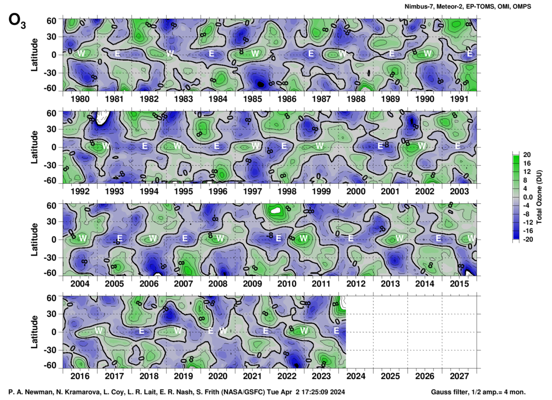
Same plot, but for 60S-60N: High-res PDF version, and png.
Daily total ozone (last 3 years) from TOMS/OMI versus latitude (deseasonalized)
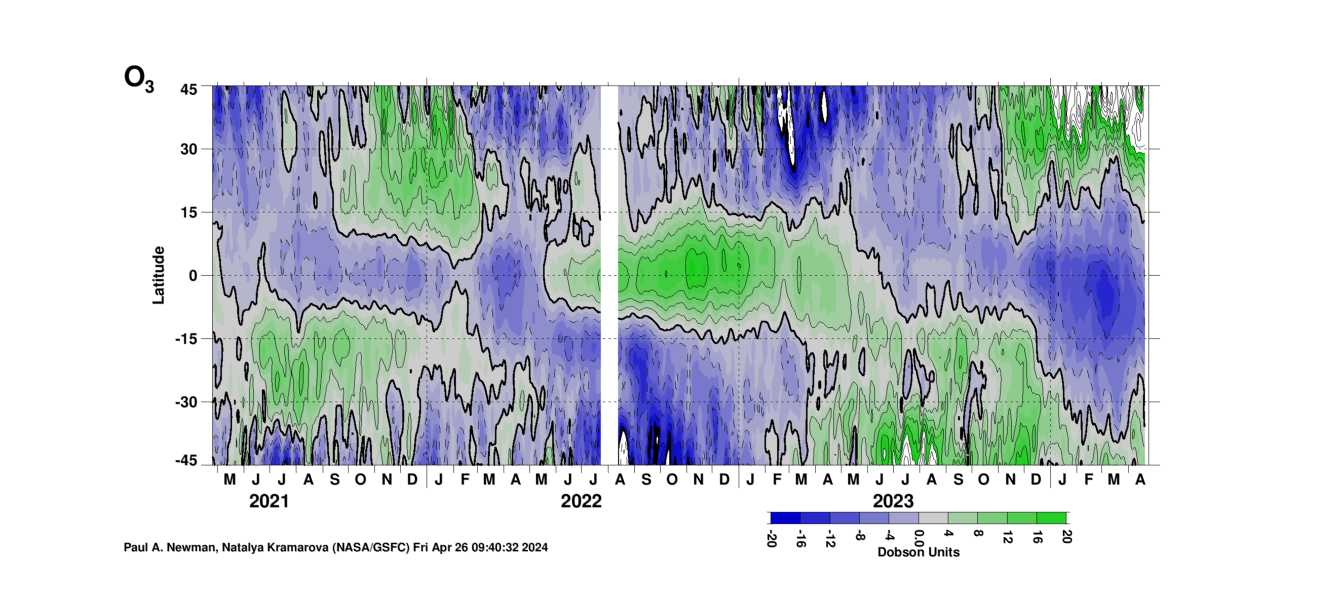
Total ozone versus latitude for daily values. The plot is generated by: 1) reading in 3-years of daily zonal mean total ozone, 2) reading in the 1979–2017 daily zonal mean data and creating a 365-day climatology, 3) subtracting this annual cycle climatology from the 3-years of daily data, 4) applying a Gaussian smoothing filter with a 6.7 day half-amplitude (i.e., high frequency features are smoothed out). Units are Dobson Units (DU).
MLS Ozone versus pressure
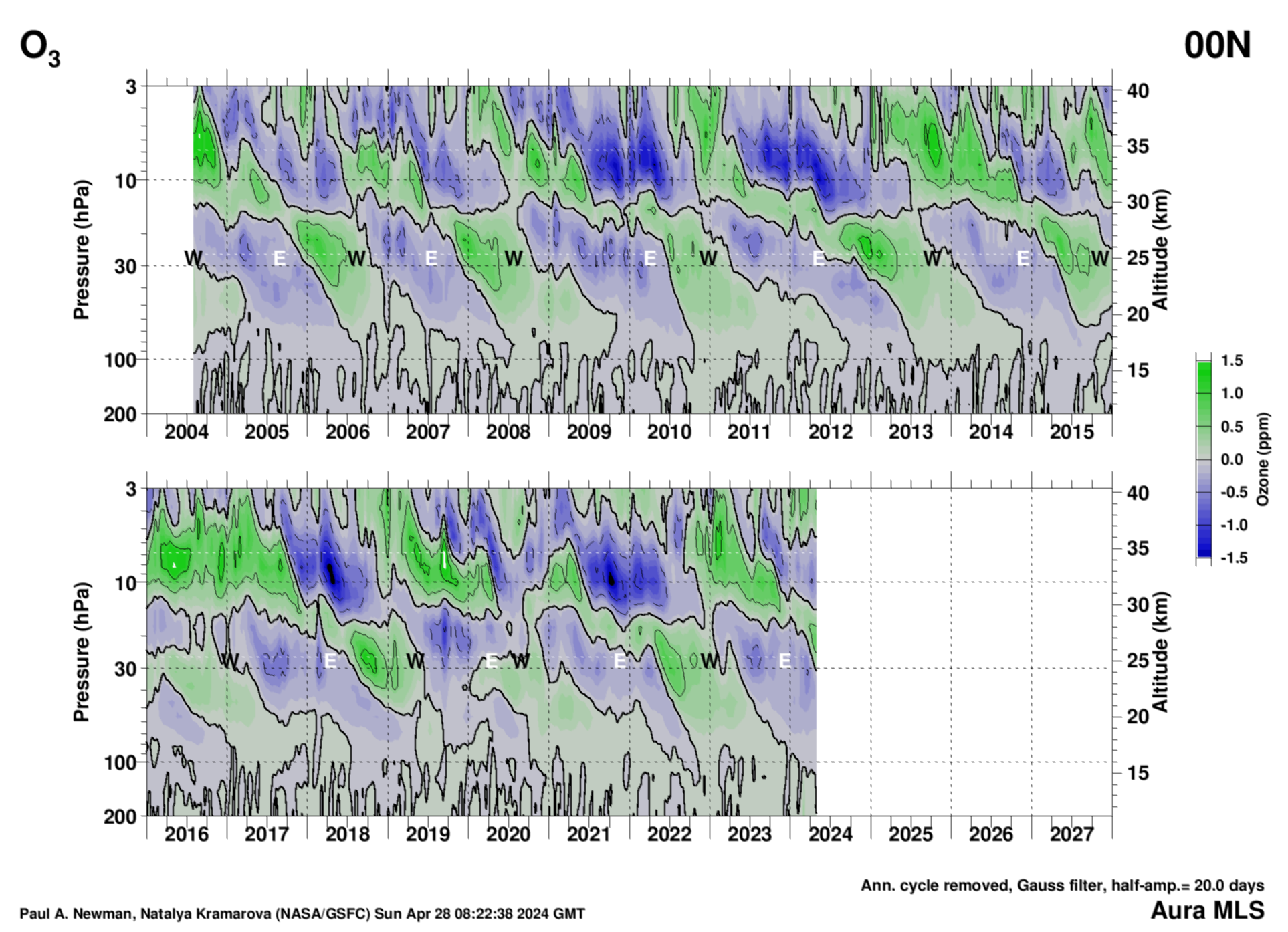
Ozone versus pressure at the equator from the NASA JPL Microwave Limb Sounder (MLS) on the NASA Aura satellite. Each day's MLS ozone is read, and all profiles within 2.5 degrees of the equator are averaged together to produce the daily ozone profiles. The annual cycle is subtracted from the profiles, and missed profiles are added by temporal linear interpolation. A Gaussian smoothing is applied (half-amplitude = 20 days) to remove higher frequency structure. The easterly (E) and westerly (W) points are as shown in the Singapore zonal winds, and are derived (see text with EOF figure) from the EOF-1 and EOF-2 phase diagram above. Units are parts per million (ppm).
Other MLS O3 profiles versus pressure and latitude.
MLS Ozone versus latitude (deseasonalized) QBO from monthly mean data versus latitude
26 hPa
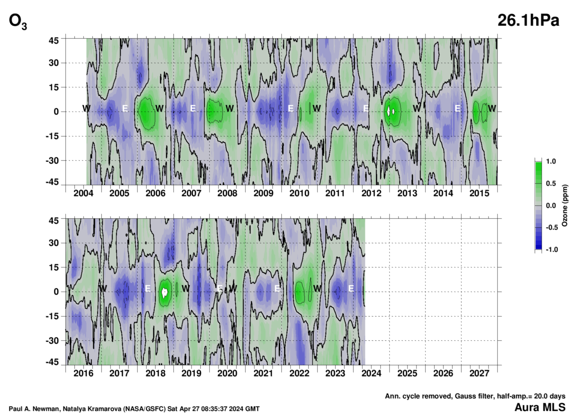
MLS ozone latitudinal profile versus time. The data are binned into 5 degree boxes from 45°S–45°N. The easterly (E) and westerly (W) points are as shown in the Singapore zonal winds, and are derived (see text with EOF figure) from the EOF-1 and EOF-2 phase diagram above. Units are parts per million (ppmv).
Other MLS O3 profiles versus pressure and latitude.
Water (H2O)
MLS water versus pressure
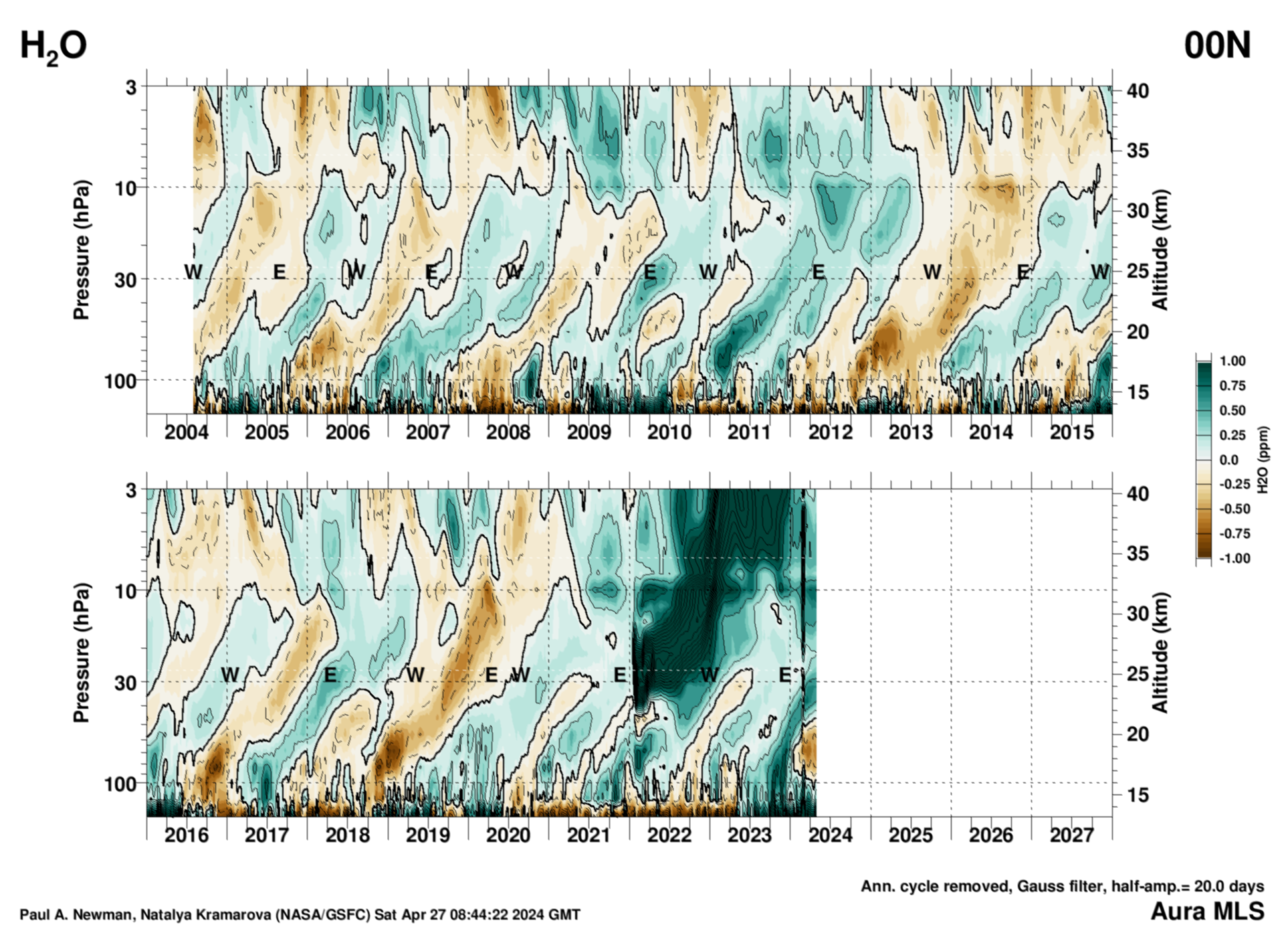
Water versus pressure at the equator from the NASA JPL Microwave Limb Sounder (MLS) on the NASA Aura satellite. Each day's MLS water is read, and all profiles within 2.5 degrees of the equator are averaged together to produce the daily water profiles. The annual cycle is subtracted from the profiles, and missed profiles are added by temporal linear interpolation. A Gaussian smoothing is applied (half-amplitude = 20 days) to remove higher frequency structure. The easterly (E) and westerly (W) points are as shown in the Singapore zonal winds, and are derived (see text with EOF figure) from the EOF-1 and EOF-2 phase diagram above. Units are parts per million (ppm).
Other MLS H2O profiles versus pressure and latitude.
MLS water versus latitude (deseasonalized) QBO from monthly mean data versus latitude
26 hPa
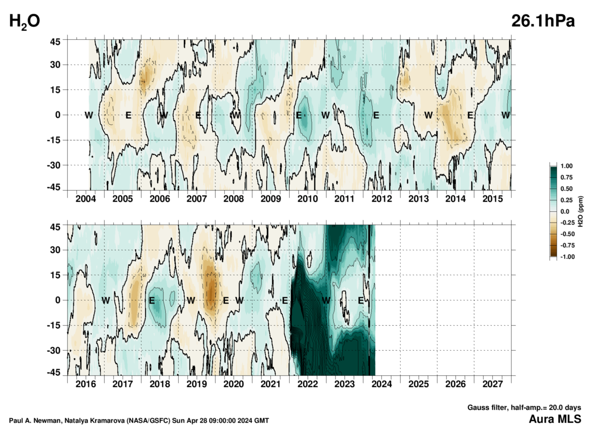
MLS water latitudinal profile versus time. The data are binned into 5 degree boxes from 45°S–45°N. A Gaussian smoothing is applied (half-amplitude = 20 days) to remove higher frequency structure. The easterly (E) and westerly (W) points are as shown in the Singapore zonal winds, and are derived (see text with EOF figure) from the EOF-1 and EOF-2 phase diagram above. Units are parts per million (ppmv). Units are parts per million (ppm).
Other MLS H2O profiles versus pressure and latitude.
QBO movie
Data Links
-
Singapore radiosondes from Meteorological Service Singapore Upper Air Observatory (station code 48698).
Global meteorological data from the Modern-Era Retrospective analysis for Research and Applications, Version-2 (MERRA-2)
Total column ozone data from the TOMS/OMI/OMPS series of instruments.
Vertical profile data from the NASA JPL Microwave Limb Sounder (MLS) on the NASA Aura satellite.
Some Related External links
QBOi — ; Towards Improving the Quasi-Biennial Oscillation in Global Climate Models
Freie Universität of Berlin QBO web page (data and figures).
NCEP Climate Prediction Center (CPC) Monthly and Atmospheric Indices including QBO
Final Note
All plots on this web site are freely available for distribution and use in presentations and publications. If used, please acknowledge NASA, this page, and the data source(s). E.g., the NASA GMAO's MERRA-2 assimilation data.

- NASA Official: Dr. Leslie R. Lait
- Web Content: Dr. Paul Newman
- Last Updated: 2019-06-10